Time Series
This section of the user guide provides an overview of some of the time series capabilities available in Streaming Expressions and Math Expressions.
Time Series Aggregation
The timeseries function performs fast, distributed time
series aggregation leveraging Solr’s built-in faceting and date math capabilities.
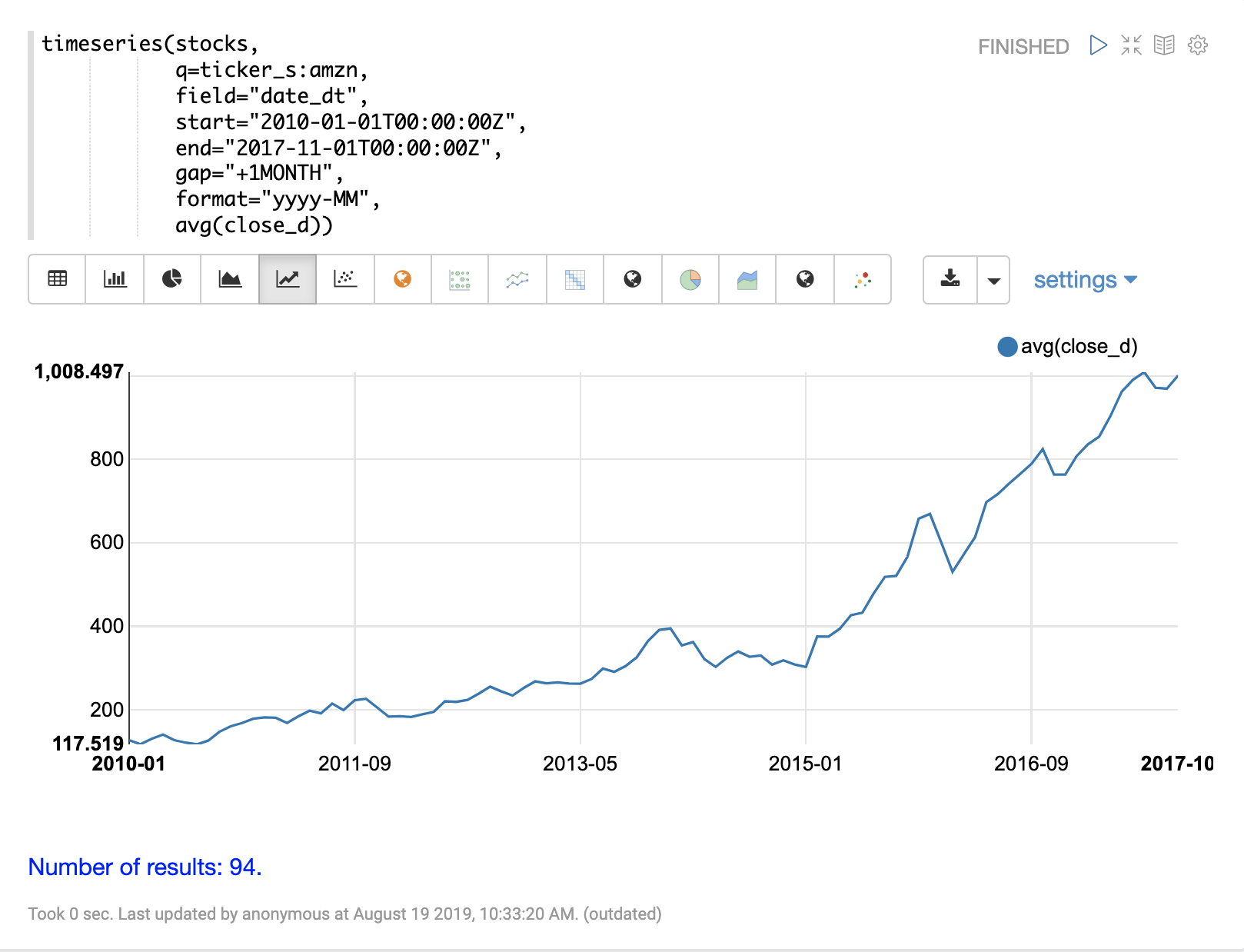
The example below performs a monthly time series aggregation over a collection of daily stock price data. In this example the average monthly closing price is calculated for the stock ticker AMZN between a specific date range.
timeseries(stocks,
           q=ticker_s:amzn,
           field="date_dt",
           start="2010-01-01T00:00:00Z",
           end="2017-11-01T00:00:00Z",
           gap="+1MONTH",
           format="YYYY-MM",
           avg(close_d))
When this expression is sent to the /stream handler it responds with:
{
  "result-set": {
    "docs": [
      {
        "date_dt": "2010-01",
        "avg(close_d)": 127.42315789473685
      },
      {
        "date_dt": "2010-02",
        "avg(close_d)": 118.02105263157895
      },
      {
        "date_dt": "2010-03",
        "avg(close_d)": 130.89739130434782
      },
      {
        "date_dt": "2010-04",
        "avg(close_d)": 141.07
      },
      {
        "date_dt": "2010-05",
        "avg(close_d)": 127.606
      },
      {
        "date_dt": "2010-06",
        "avg(close_d)": 121.66681818181816
      },
      {
        "date_dt": "2010-07",
        "avg(close_d)": 117.5190476190476
      }
]}}
Using Zeppelin-Solr this time series can be visualized using a line chart.
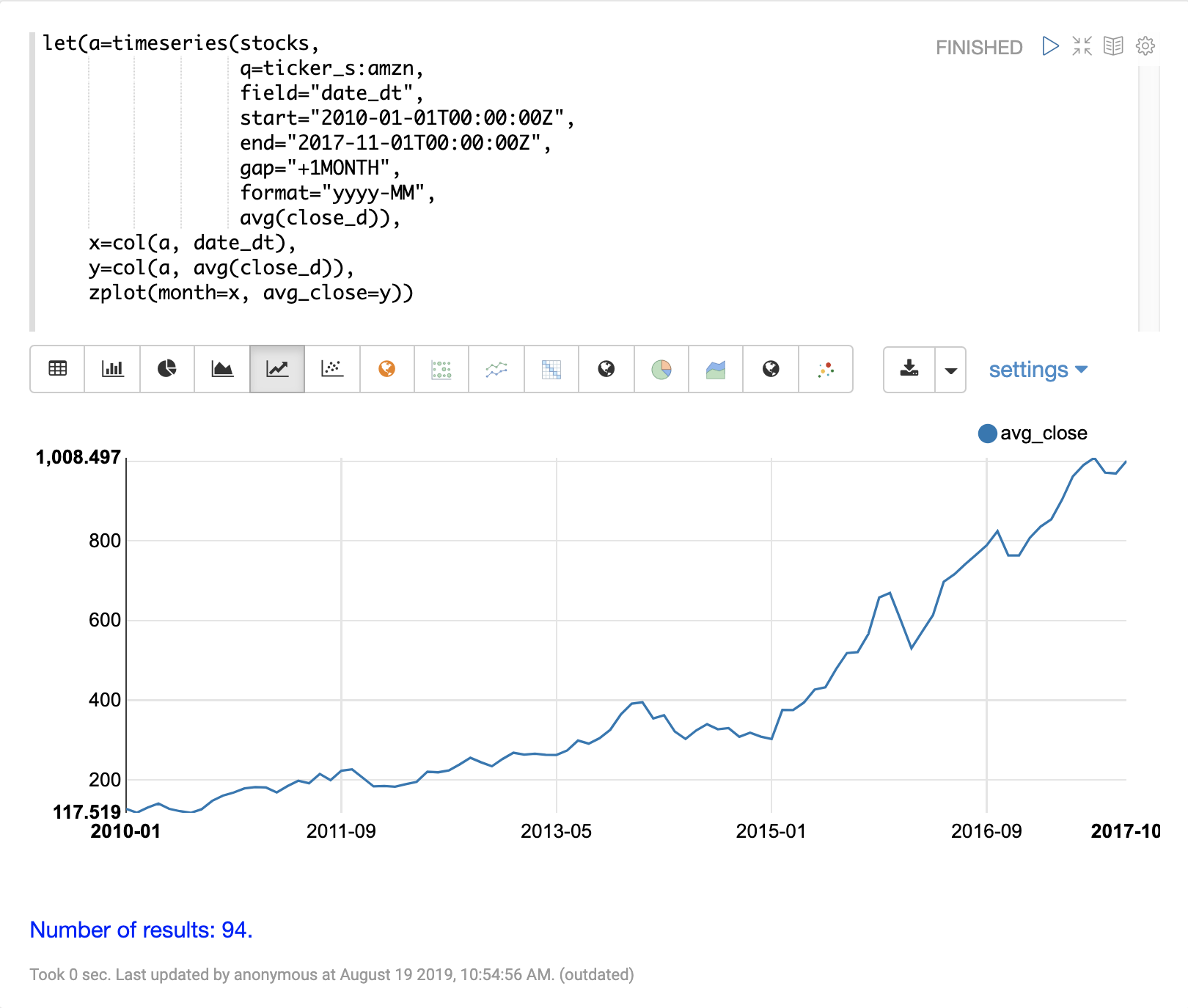
Vectorizing the Time Series
Before a time series can be smoothed or modeled the data will need to be vectorized.
The col function can be used
to copy a column of data from a list of tuples into an array.
The expression below demonstrates the vectorization of the date_dt and avg(close_d) fields.
The zplot function is then used to plot the months on the x-axis and the average closing prices on the y-axis.
Smoothing
Time series smoothing is often used to remove the noise from a time series and help spot the underlying trend. The math expressions library has three sliding window approaches for time series smoothing. These approaches use a summary value from a sliding window of the data to calculate a new set of smoothed data points.
The three sliding window functions are lagging indicators, which means they don’t start to move in the direction of the trend until the trend effects the summary value of the sliding window. Because of this lagging quality these smoothing functions are often used to confirm the direction of the trend.
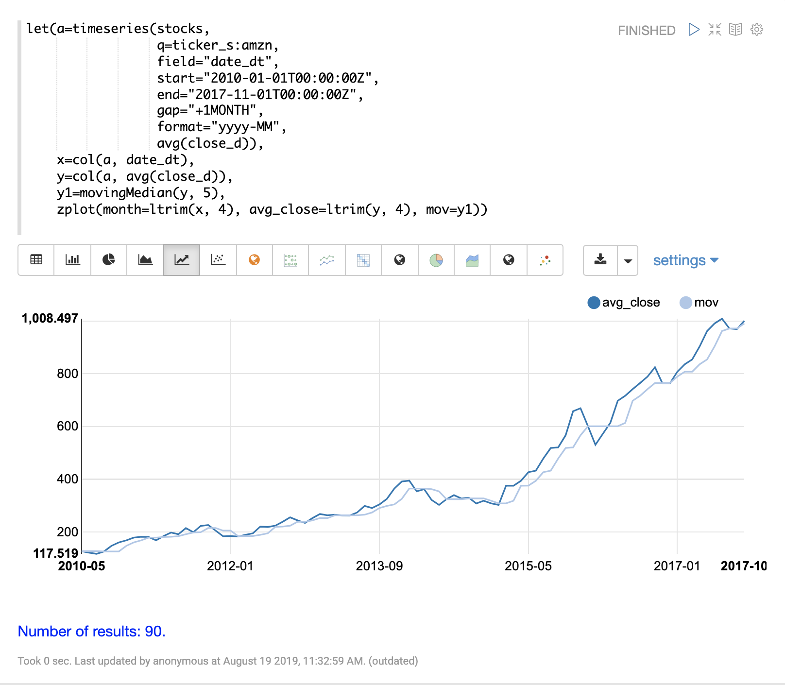
Moving Average
The movingAvg function computes a simple moving average over a sliding window of data.
The example below generates a time series, vectorizes the avg(close_d) field and computes the
moving average with a window size of 5.
The moving average function returns an array that is of shorter length then the original vector. This is because results are generated only when a full window of data is available for computing the average. With a window size of five the moving average will begin generating results at the 5th value. The prior values are not included in the result.
The zplot function is then used to plot the months on the x-axis, and the average close and moving
average on the y-axis. Notice that the ltrim function is used to trim the first 4 values from
the x-axis and the average closing prices. This is done to line up the three arrays so they start
from the 5th value.

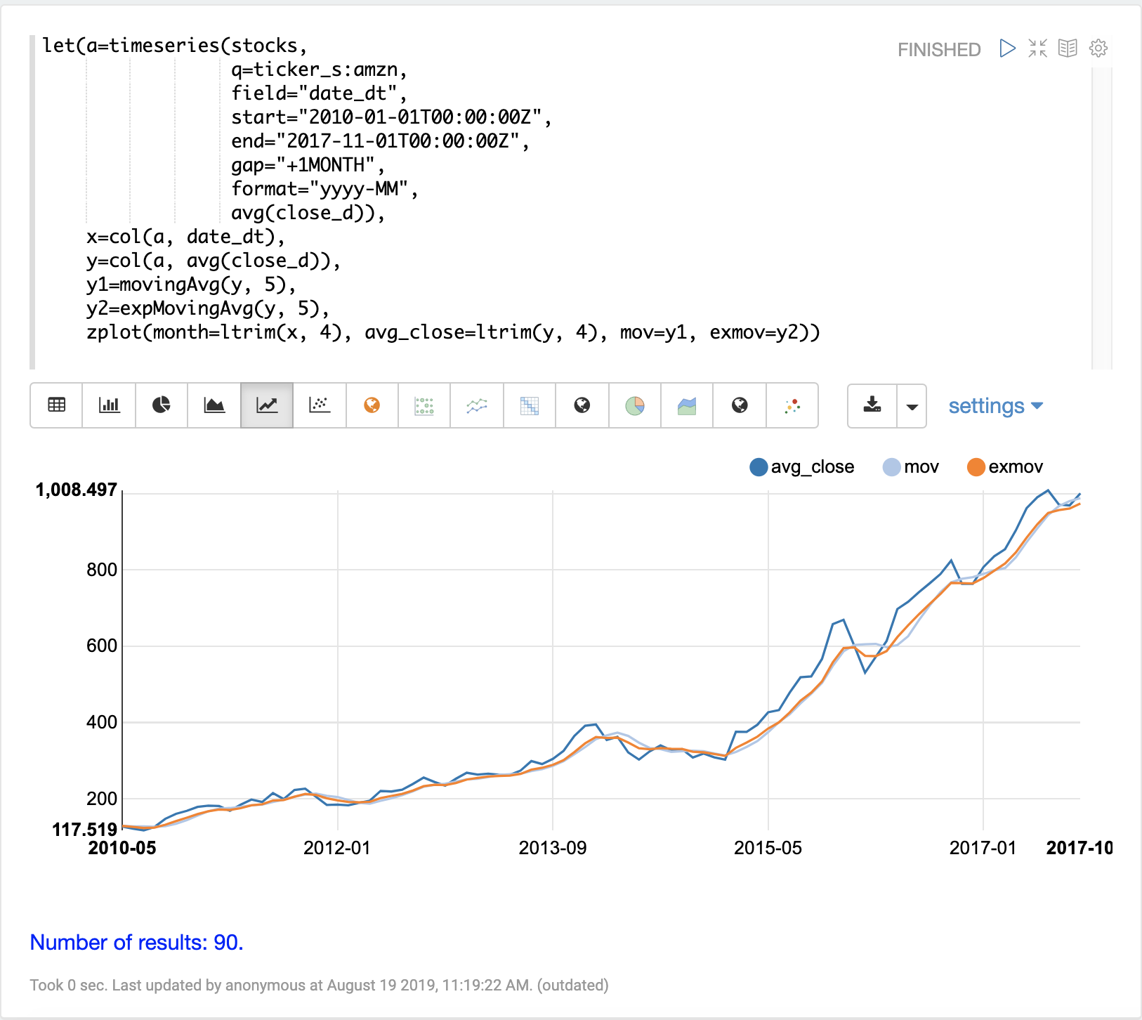
Exponential Moving Average
The expMovingAvg function uses a different formula for computing the moving average that
responds faster to changes in the underlying data. This means that it is
less of a lagging indicator than the simple moving average.
Below is an example that computes a moving average and exponential moving average and plots them along with the original y values. Notice how the exponential moving average is more sensitive to changes in the y values.
Moving Median
The movingMedian function uses the median of the sliding window rather than the average.
In many cases the moving median will be more robust to outliers than moving averages.
Below is an example computing the moving median:
Differencing
Differencing can be used to make a time series stationary by removing the trend or seasonality from the series.
First Difference
The technique used in differencing is to use the difference between values rather than the original values. The first difference takes the difference between a value and the value that came directly before it. The first difference is often used to remove the trend from a time series.
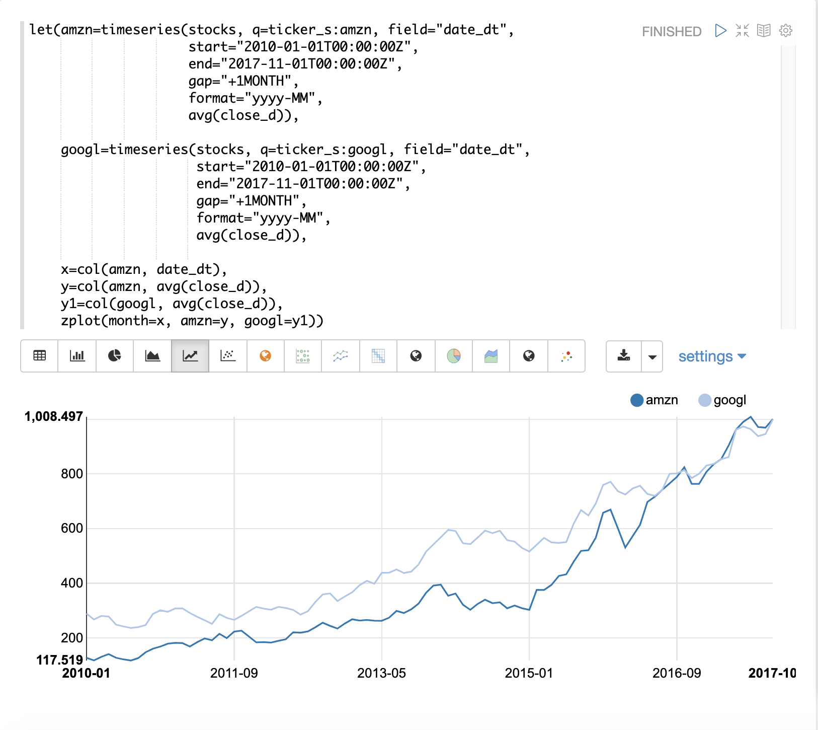
The examples below uses the first difference to make two time series stationary so they can be compared without the trend.
In this example we’ll be comparing the average monthly closing price for two stocks: Amazon and Google. The image below plots both time series before differencing is applied.
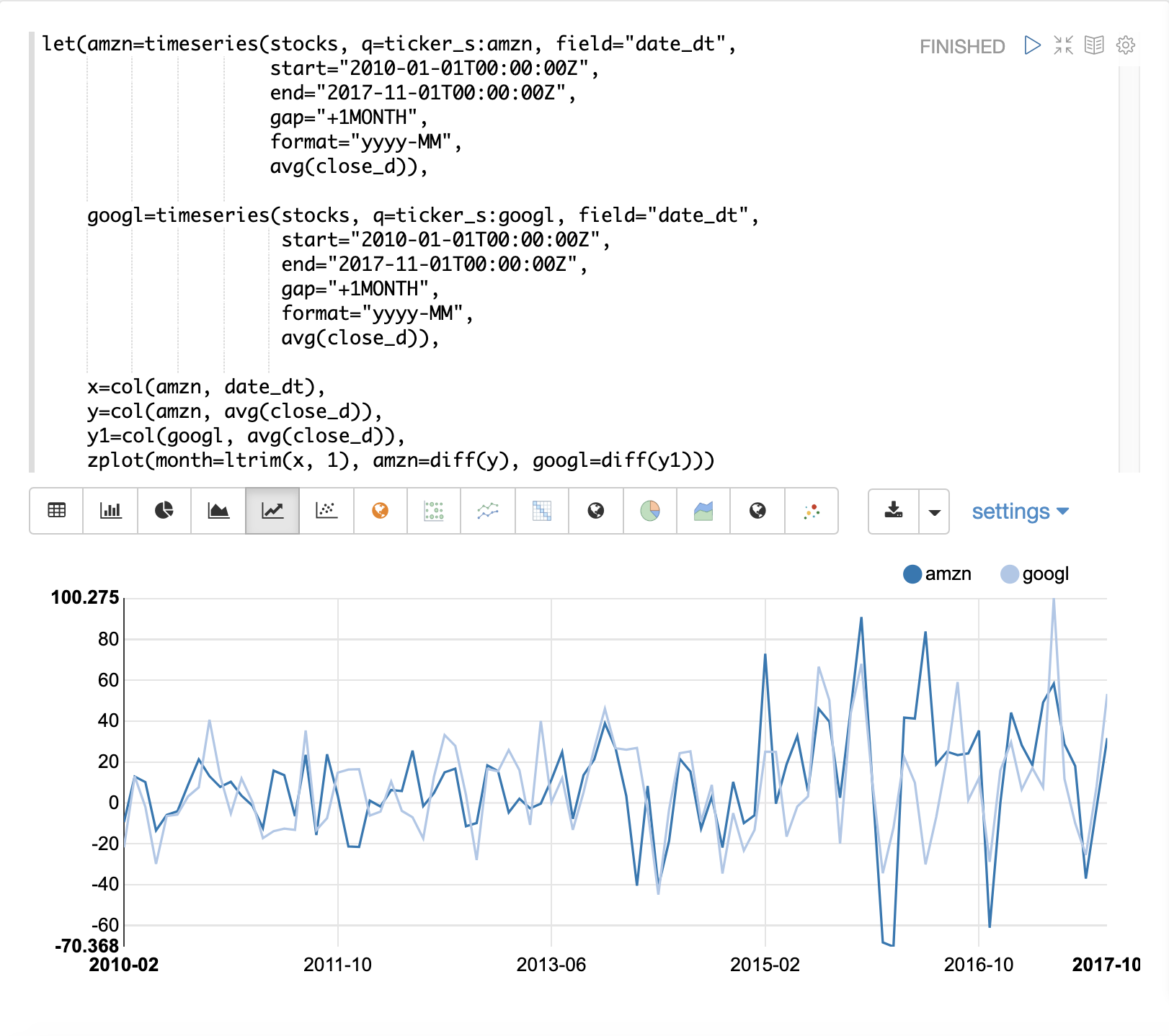
In the next example the diff function is applied to both time series inside the zplot function.
The diff can be applied inside the zplot function or like any other function inside of the let
function.
Notice that both time series now have the trend removed and the monthly movements of the stock price can be studied without being influenced by the trend.
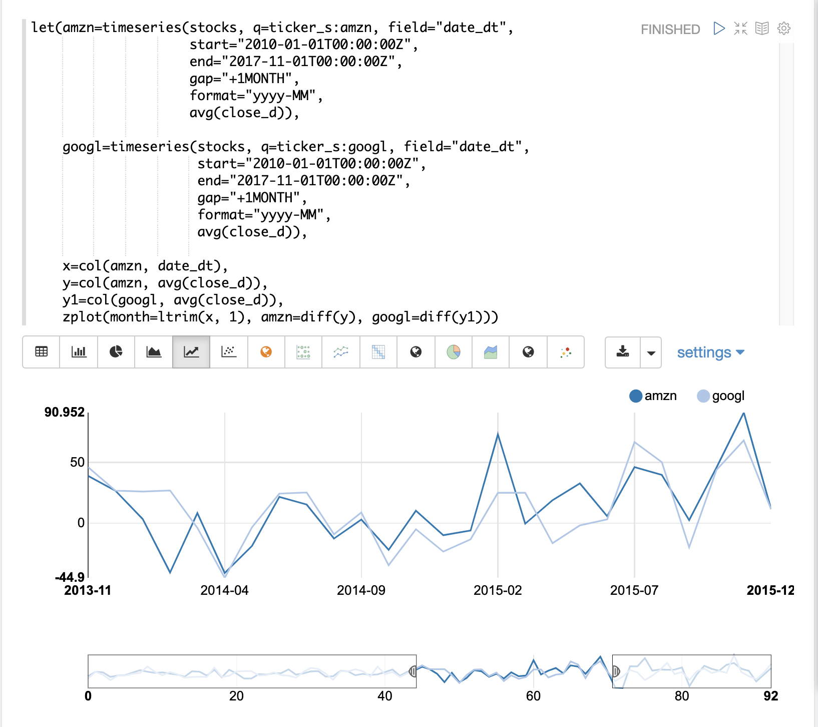
In the next example the zoom function of the time series visualization is used to zoom into a specific
range of months. This allows for closer inspection of the data. With closer inspection of the data there appears
to be some correlation between the monthly movements of the two stocks.
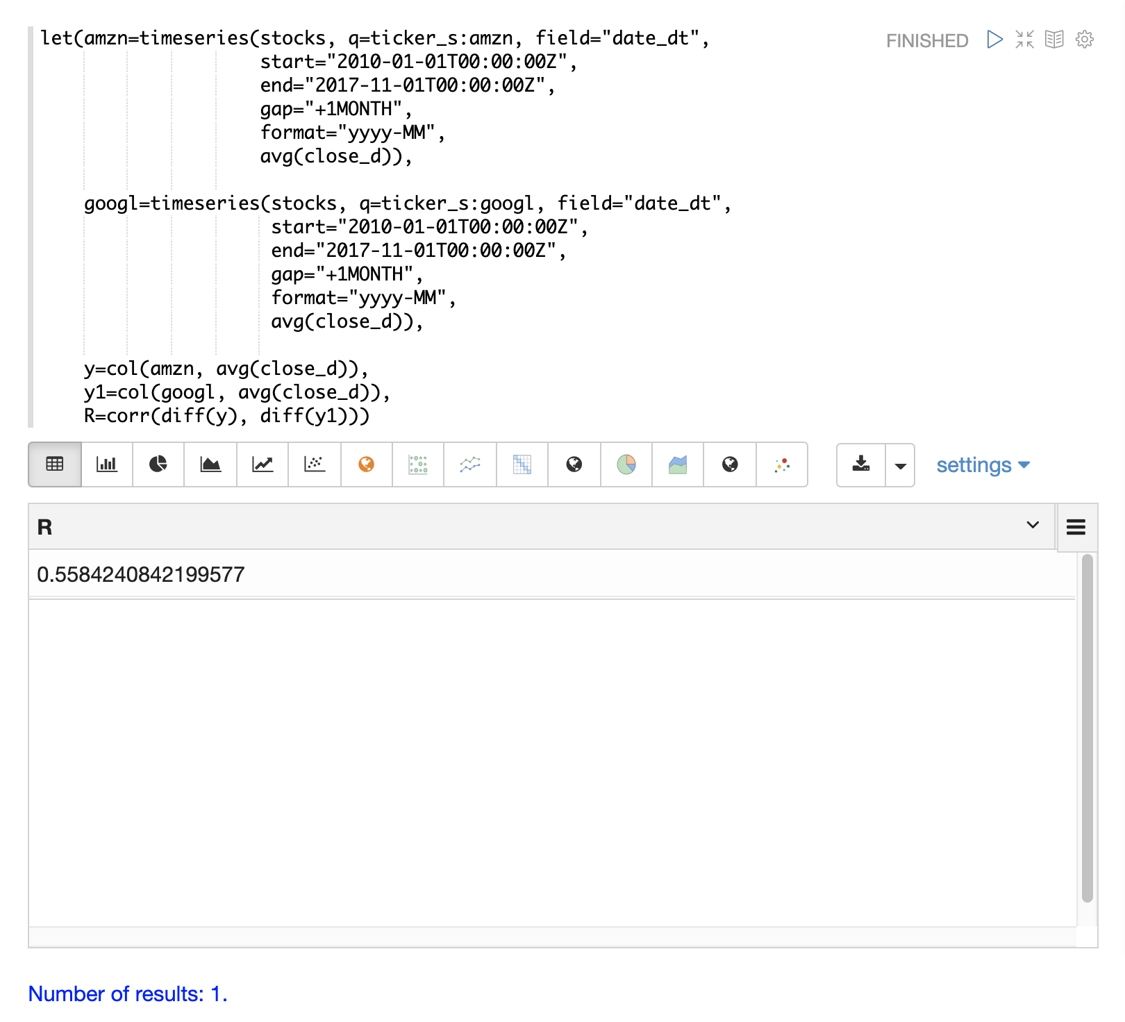
In the final example the differenced time series are correlated with the corr function.
Lagged Differences
The diff function has an optional second parameter to specify a lag in the difference.
If a lag is specified the difference is taken between a value and the value at a specified
lag in the past. Lagged differences are often used to remove seasonality from a time series.
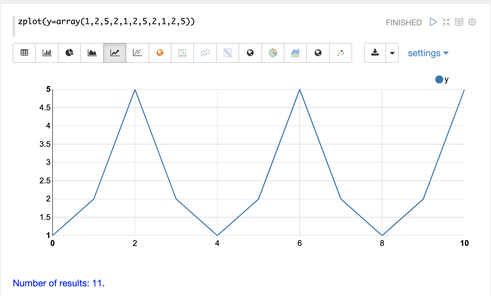
The simple example below demonstrates how lagged differencing works. Notice that the array in the example follows a simple repeated pattern. This type of pattern is often displayed with seasonality.
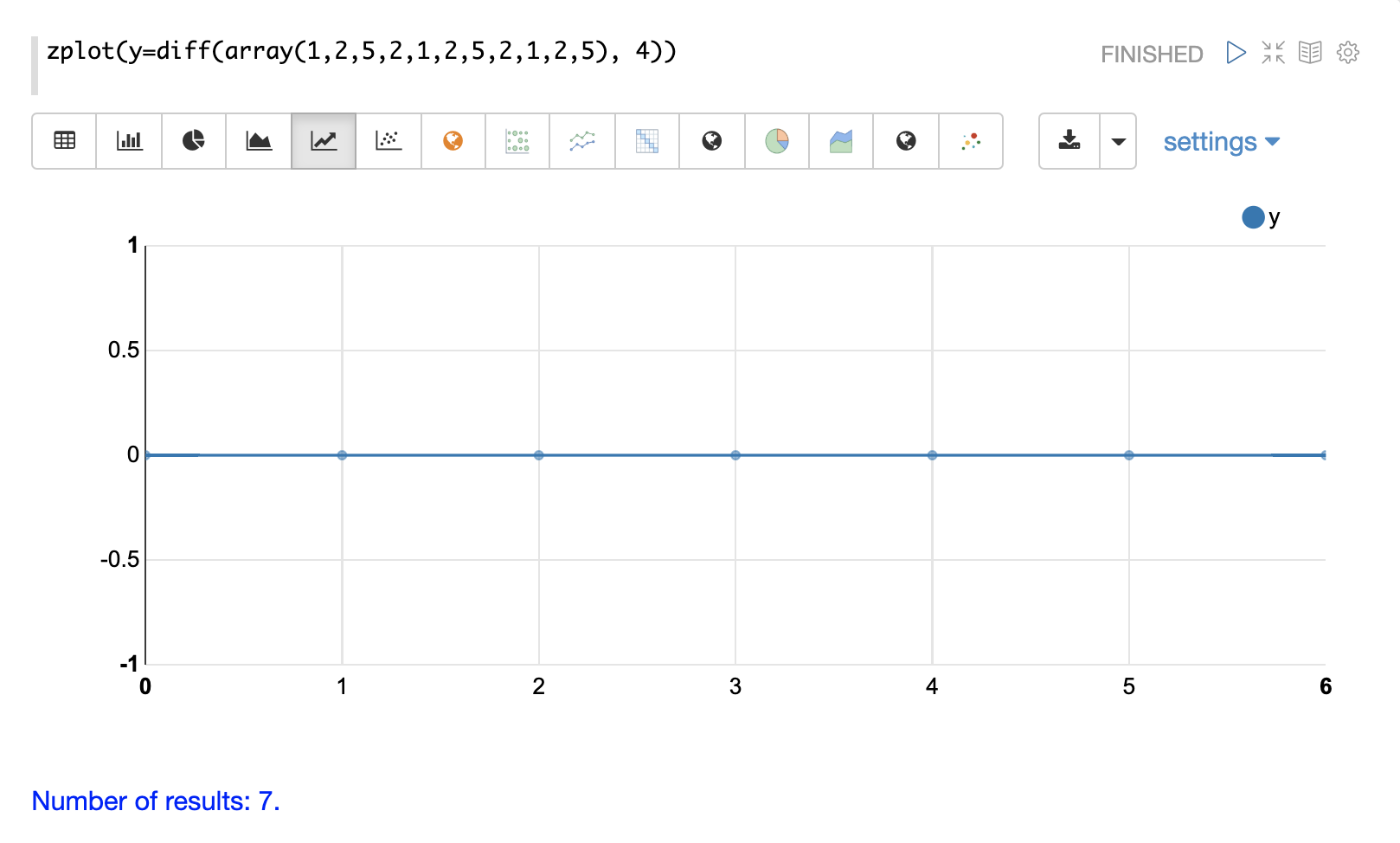
In this example we remove this pattern using
the diff function with a lag of 4. This will subtract the value lagging four indexes
behind the current index. Notice that the result set size is the original array size minus the lag.
This is because the diff function only returns results for values where the lag of 4
is possible to compute.
Anomaly Detection
The movingMAD (moving mean absolute deviation) function can be used to surface anomalies
in a time series by measuring dispersion (deviation from the mean) within a sliding window.
The movingMAD function operates in a similar manner as a moving average, except it
measures the mean absolute deviation within the window rather than the average. By
looking for unusually high or low dispersion we can find anomalies in the time
series.
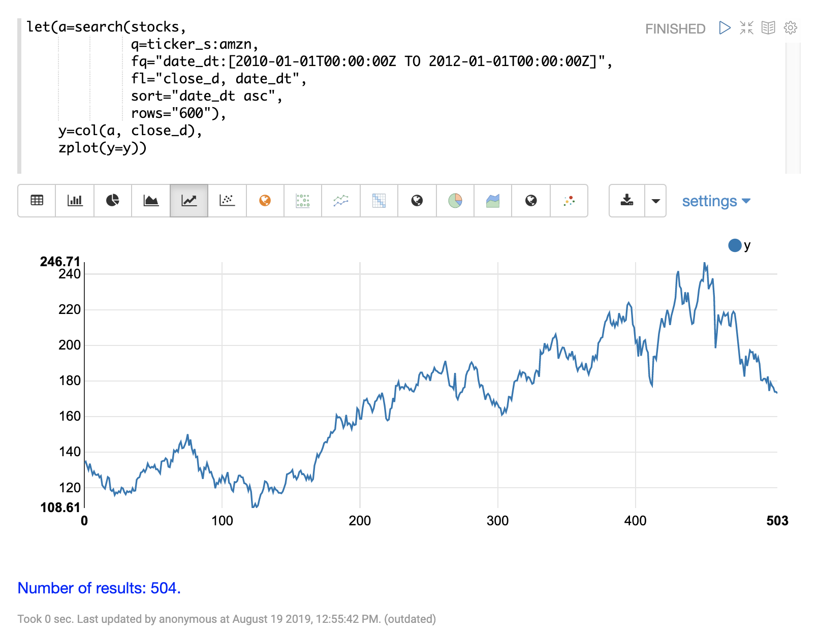
For this example we’ll be working with daily stock prices for Amazon over a two year period. The daily stock data will provide a larger data set to study.
In the example below the search expression is used to return the daily closing price
for the ticker AMZN over a two year period.
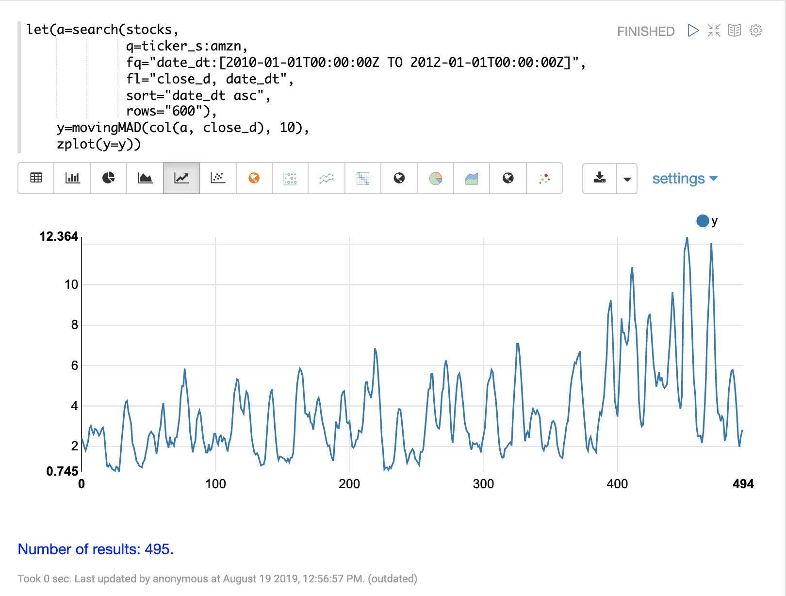
The next step is to apply the movingMAD function to the data to calculate
the moving mean absolute deviation over a 10 day window. The example below shows the function being
applied and visualized.
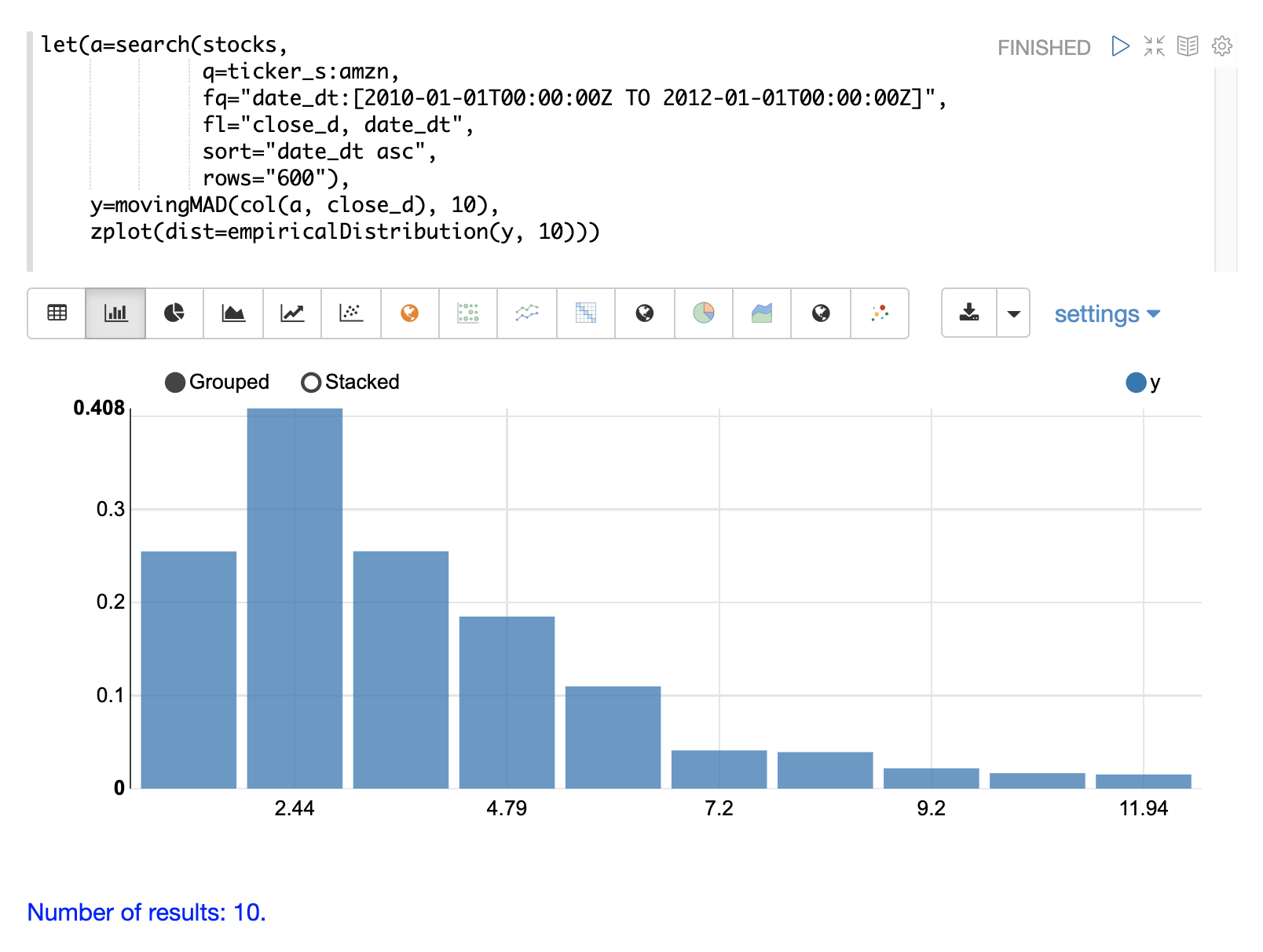
Once the moving MAD has been calculated we can visualize the distribution of dispersion
with the empiricalDistribution function. The example below plots the empirical
distribution with 10 bins, creating a 10 bin histogram of the dispersion of the
time series.
This visualization shows that most of the mean absolute deviations fall between 0 and 9.2 with the mean of the final bin at 11.94.
The final step is to detect outliers in the series using the outliers function.
The outliers function uses a probability distribution to find outliers in a numeric vector.
The outliers function takes four parameters:
Probability distribution
Numeric vector
Low probability threshold
High probability threshold
List of results that the numeric vector was selected from
The outliers function iterates the numeric vector and uses the probability
distribution to calculate the cumulative probability of each value. If the cumulative
probability is below the low probability threshold or above the high threshold it considers
the value an outlier. When the outliers function encounters an outlier it returns
the corresponding result from the list of results provided by the fifth parameter.
It also includes the cumulative probability and the value of the outlier.
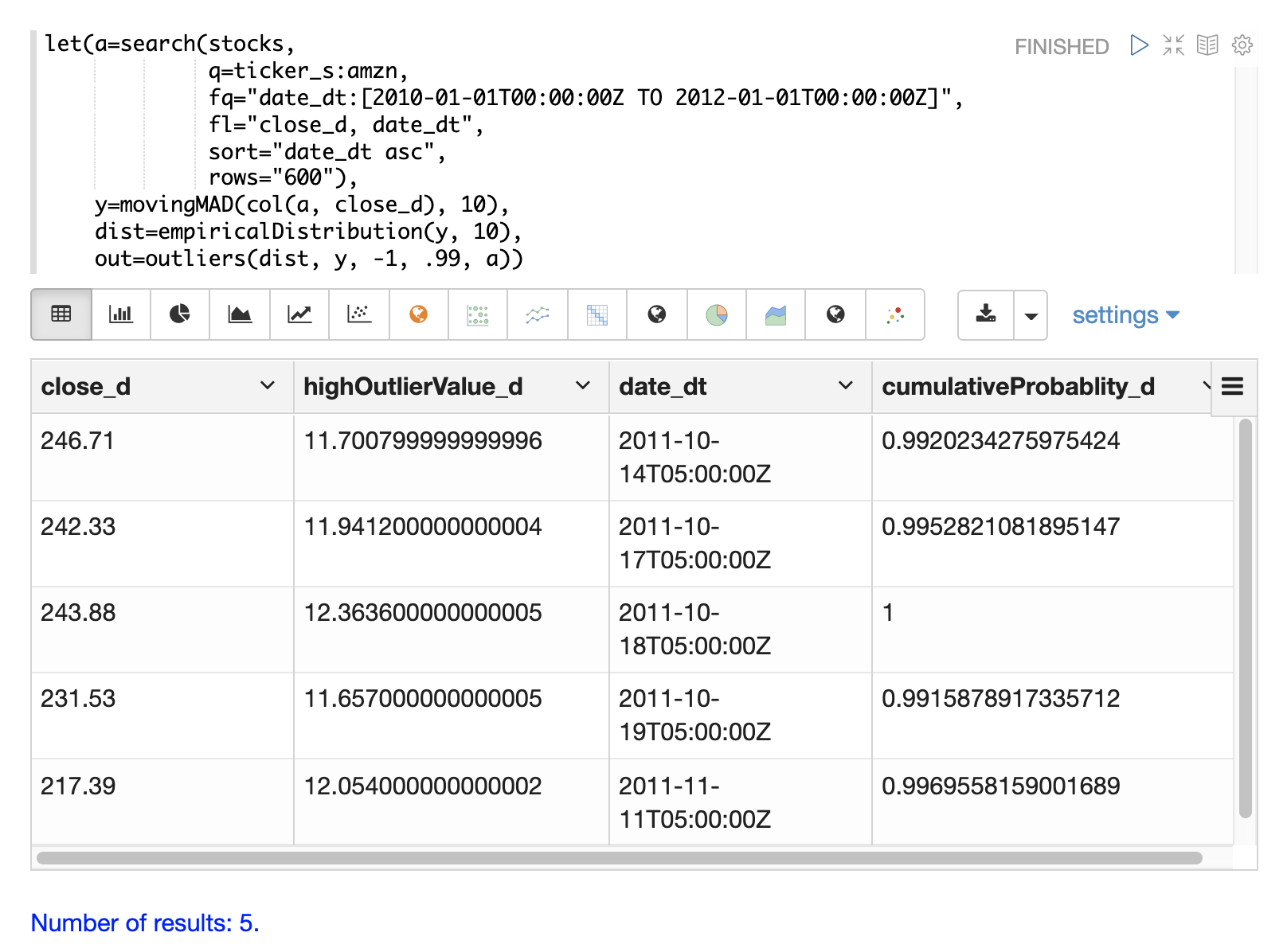
The example below shows the outliers function applied to the Amazon stock
price data set. The empirical distribution of the moving mean absolute deviation is
the first parameter. The vector containing the moving mean absolute
deviations is the second parameter. -1 is the low and .99 is the high probability
thresholds. -1 means that low outliers will not be considered. The final parameter
is the original result set containing the close_d and date_dt fields.
The output of the outliers function contains the results where an outlier was detected.
In this case 5 results above the .99 probability threshold were detected.
Modeling
Math expressions support in Solr includes a number of functions that can be used to model a time series. These functions include linear regression, polynomial and harmonic curve fitting, loess regression, and KNN regression.
Each of these functions can model a time series and be used for interpolation (predicting values within the dataset) and several can be used for extrapolation (predicting values beyond the data set).
The various regression functions are covered in detail in the Linear Regression, Curve Fitting and Machine Learning sections of the user guide.
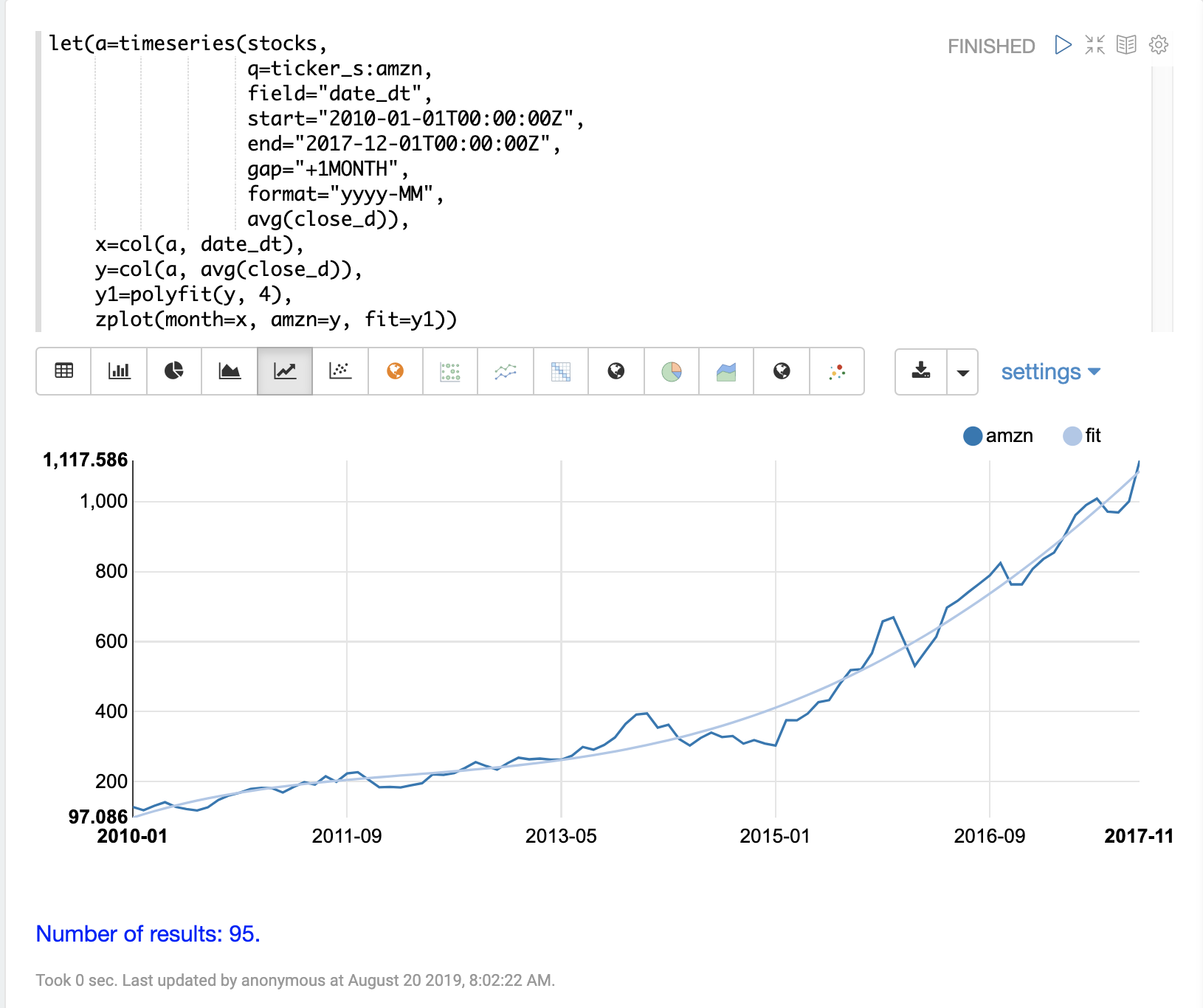
The example below uses the polyfit function (polynomial regression) to
fit a non-linear model to a time series. The data set being used is the
monthly average closing price for Amazon over an eight year period.
In this example the polyfit function returns a fitted model for the y
axis, which is the average monthly closing prices, using a 4 degree polynomial.
The degree of the polynomial determines the number of curves in the
model. The fitted model is set to the variable y1. The fitted model
is then directly plotted with zplot along with the original y
values.
The visualization shows the smooth line fit through the average closing price data.
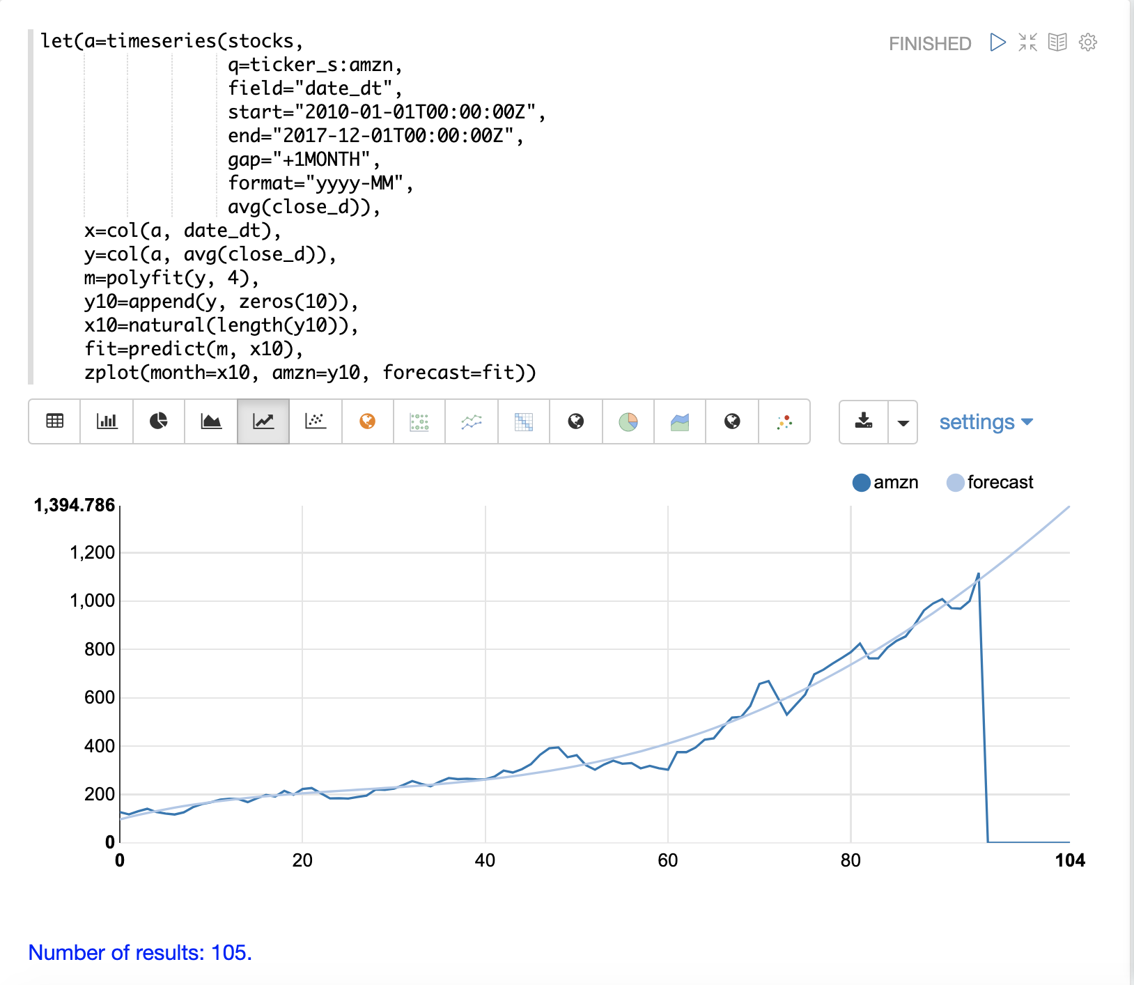
Forecasting
The polyfit function can also be used to extrapolate a time series to forecast
future stock prices. The example below demonstrates a 10 month forecast.
In the example the polyfit function fits a model to the y-axis and the model
is set to the variable m.
Then to create a forecast 10 zeros are appended
to the y-axis to create new vector called y10.
Then a new x-axis is created using
the natural function which returns a sequence of whole numbers 0 to the length of y10.
The new x-axis is stored in the variable x10.
The predict function uses the fitted model to predict values for the new x-axis stored in
variable x10.
The zplot function is then used to plot the x10 vector on the x-axis and the y10 vector and extrapolated
model on the y-axis. Notice that the y10 vector drops to zero where the observed data
ends, but the forecast continues along the fitted curve
of the model.