Linear Regression
The math expressions library supports simple and multivariate linear regression.
Simple Linear Regression
The regress function is used to build a linear regression model
between two random variables. Sample observations are provided with two
numeric arrays. The first numeric array is the independent variable and
the second array is the dependent variable.
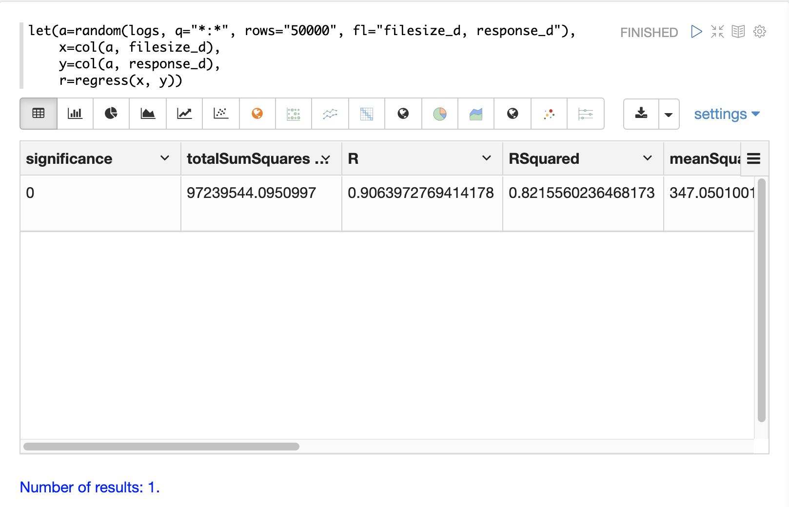
In the example below the random function selects 50000 random samples each containing
the fields filesize_d and response_d. The two fields are vectorized
and stored in variables x and y. Then the regress function performs a regression
analysis on the two numeric arrays.
The regress function returns a single tuple with the results of the regression
analysis.
let(a=random(logs, q="*:*", rows="50000", fl="filesize_d, response_d"),
    x=col(a, filesize_d),
    y=col(a, response_d),
    r=regress(x, y))
Note that in this regression analysis the value of RSquared is .75. This means that changes in
filesize_d explain 75% of the variability of the response_d variable:
{
  "result-set": {
    "docs": [
      {
        "significance": 0,
        "totalSumSquares": 96595678.64838874,
        "R": 0.9052835767815126,
        "RSquared": 0.8195383543903288,
        "meanSquareError": 348.6502485633668,
        "intercept": 55.64040842391729,
        "slopeConfidenceInterval": 0.0000822026526346821,
        "regressionSumSquares": 79163863.52071753,
        "slope": 0.019984612363694493,
        "interceptStdErr": 1.6792610845256566,
        "N": 50000
      },
      {
        "EOF": true,
        "RESPONSE_TIME": 344
      }
    ]
  }
}
The diagnostics can be visualized in a table using Zeppelin-Solr.
Prediction
The predict function uses the regression model to make predictions.
Using the example above the regression model can be used to predict the value
of response_d given a value for filesize_d.
In the example below the predict function uses the regression analysis to predict
the value of response_d for the filesize_d value of 40000.
let(a=random(logs, q="*:*", rows="5000", fl="filesize_d, response_d"),
    x=col(a, filesize_d),
    y=col(a, response_d),
    r=regress(x, y),
    p=predict(r, 40000))
When this expression is sent to the /stream handler it responds with:
{
  "result-set": {
    "docs": [
      {
        "p": 748.079241022975
      },
      {
        "EOF": true,
        "RESPONSE_TIME": 95
      }
    ]
  }
}
The predict function can also make predictions for an array of values. In this
case it returns an array of predictions.
In the example below the predict function uses the regression analysis to
predict values for each of the 5000 samples of filesize_d used to generate the model.
In this case 5000 predictions are returned.
let(a=random(logs, q="*:*", rows="5000", fl="filesize_d, response_d"),
    x=col(a, filesize_d),
    y=col(a, response_d),
    r=regress(x, y),
    p=predict(r, x))
When this expression is sent to the /stream handler it responds with:
{
  "result-set": {
    "docs": [
      {
        "p": [
          742.2525322514165,
          709.6972488729955,
          687.8382568904871,
          820.2511324266264,
          720.4006432289061,
          761.1578181053039,
          759.1304101159126,
          699.5597256337142,
          742.4738911248204,
          769.0342605881644,
          746.6740473150268
          ]
      },
      {
        "EOF": true,
        "RESPONSE_TIME": 113
      }
    ]
  }
}
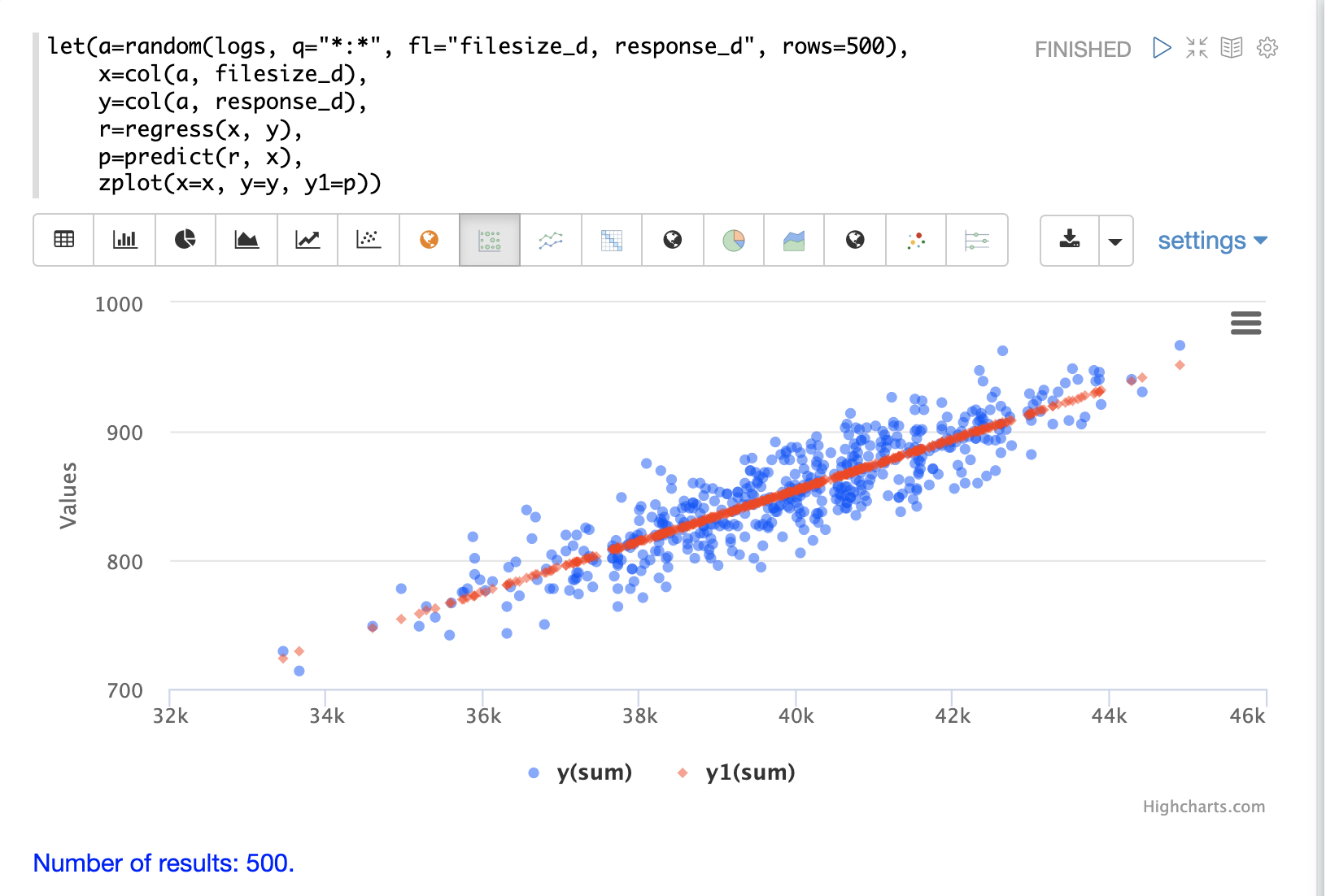
Regression Plot
Using zplot and the Zeppelin-Solr interpreter we can visualize both the observations and the predictions in
the same scatter plot.
In the example below zplot is plotting the filesize_d observations on the
x-axis, the response_d observations on the y-axis and the predictions on the y1-axis.
Residuals
The difference between the observed value and the predicted value is known as the residual. There isn’t a specific function to calculate the residuals but vector math can used to perform the calculation.
In the example below the predictions are stored in variable p. The ebeSubtract
function is then used to subtract the predictions
from the actual response_d values stored in variable y. Variable e contains
the array of residuals.
let(a=random(logs, q="*:*", rows="500", fl="filesize_d, response_d"),
    x=col(a, filesize_d),
    y=col(a, response_d),
    r=regress(x, y),
    p=predict(r, x),
    e=ebeSubtract(y, p))
When this expression is sent to the /stream handler it responds with:
{
  "result-set": {
    "docs": [
      {
        "e": [
          31.30678554491226,
          -30.292830927953446,
          -30.49508862647258,
          -30.499884780783532,
          -9.696458959319784,
          -30.521563961535094,
          -30.28380938033081,
          -9.890289849359306,
          30.819723560583157,
          -30.213178859683012,
          -30.609943619066826,
          10.527700442607625,
          10.68046928406568
          ]
      },
      {
        "EOF": true,
        "RESPONSE_TIME": 113
      }
    ]
  }
}
Residual Plot
Using zplot and Zeppelin-Solr we can visualize the residuals with
a residuals plot. The example residual plot below plots the predicted value on the
x-axis and the error of the prediction on the y-axis.
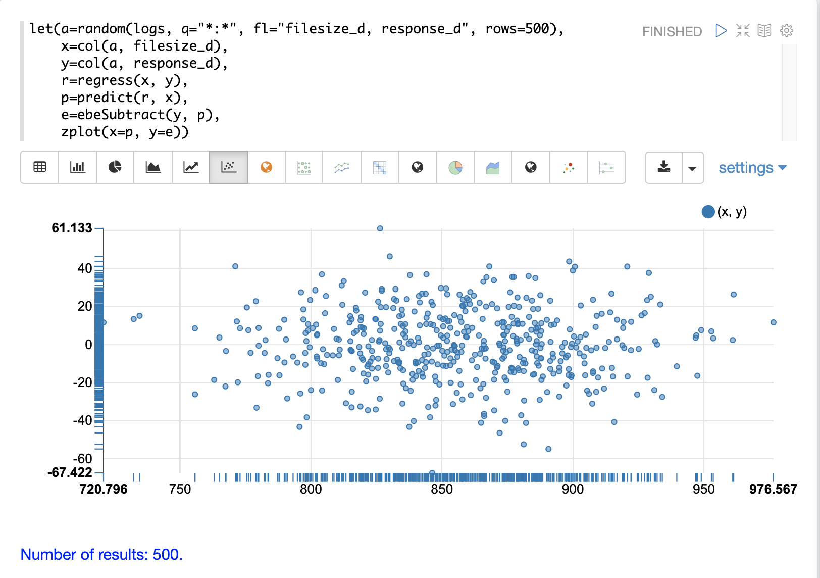
The residual plot can be used to interpret reliability of the model. Three things to look for are:
- Do the residuals appear to be normally distributed with a mean of 0? This makes it easier to interpret the results of the model to determine if the distribution of the errors is acceptable for predictions. It also makes it easier to use a model of the residuals for anomaly detection on new predictions.
- Do the residuals appear to be heteroscedastic? Which means is the variance of the residuals the same across the range of predictions? By plotting the prediction on the x-axis and error on y-axis we can see if the variability stays the same as the predictions get higher. If the residuals are heteroscedastic it means that we can trust the models error to be consistent across the range of predictions.
- Is there any pattern to the residuals? If so there is likely still a signal within the data that needs to be modeled.
Multivariate Linear Regression
The olsRegress function performs a multivariate linear regression analysis. Multivariate linear
regression models the linear relationship between two or more independent variables and a dependent variable.
The example below extends the simple linear regression example by introducing a new independent variable
called load_d. The load_d variable is the load on the network while the file is being downloaded.
Notice that the two independent variables filesize_d and load_d are vectorized and stored
in the variables b and c. The variables b and c are then added as rows to a matrix. The matrix is
then transposed so that each row in the matrix represents one observation with filesize_d and service_d.
The olsRegress function then performs the multivariate regression analysis using the observation matrix as the
independent variables and the response_d values, stored in variable d, as the dependent variable.
let(a=random(testapp, q="*:*", rows="30000", fl="filesize_d, load_d, response_d"),
    x=col(a, filesize_d),
    y=col(a, load_d),
    z=col(a, response_d),
    m=transpose(matrix(x, y)),
    r=olsRegress(m, z))
Notice in the response that the RSquared of the regression analysis is 1. This means that linear relationship between
filesize_d and service_d describe 100% of the variability of the response_d variable:
{
  "result-set": {
    "docs": [
      {
        "regressionParametersStandardErrors": [
          1.7792032752524236,
          0.0000429945089590394,
          0.0008592489428291642
        ],
        "RSquared": 0.8850359458670845,
        "regressionParameters": [
          0.7318766882597804,
          0.01998298784650873,
          0.10982104952105468
        ],
        "regressandVariance": 1938.8190758686717,
        "regressionParametersVariance": [
          [
            0.014201127587649602,
            -3.326633951803927e-7,
            -0.000001732754417954437
          ],
          [
            -3.326633951803927e-7,
            8.292732891338694e-12,
            2.0407522508189773e-12
          ],
          [
            -0.000001732754417954437,
            2.0407522508189773e-12,
            3.3121477630934995e-9
          ]
        ],
        "adjustedRSquared": 0.8850282808303053,
        "residualSumSquares": 6686612.141261716
      },
      {
        "EOF": true,
        "RESPONSE_TIME": 374
      }
    ]
  }
}
Prediction
The predict function can also be used to make predictions for multivariate linear regression.
Below is an example of a single prediction using the multivariate linear regression model and a single observation.
The observation is an array that matches the structure of the observation matrix used to build the model. In this case
the first value represents a filesize_d of 40000 and the second value represents a load_d of 4.
let(a=random(logs, q="*:*", rows="5000", fl="filesize_d, load_d, response_d"),
    x=col(a, filesize_d),
    y=col(a, load_d),
    z=col(a, response_d),
    m=transpose(matrix(x, y)),
    r=olsRegress(m, z),
    p=predict(r, array(40000, 4)))
When this expression is sent to the /stream handler it responds with:
{
  "result-set": {
    "docs": [
      {
        "p": 801.7725344814675
      },
      {
        "EOF": true,
        "RESPONSE_TIME": 70
      }
    ]
  }
}
The predict function can also make predictions for more than one multivariate observation. In this scenario
an observation matrix used.
In the example below the observation matrix used to build the multivariate regression model
is passed to the predict function and it returns an array of predictions.
let(a=random(logs, q="*:*", rows="5000", fl="filesize_d, load_d, response_d"),
    x=col(a, filesize_d),
    y=col(a, load_d),
    z=col(a, response_d),
    m=transpose(matrix(x, y)),
    r=olsRegress(m, z),
    p=predict(r, m))
When this expression is sent to the /stream handler it responds with:
{
  "result-set": {
    "docs": [
      {
        "p": [
          917.7122088913725,
          900.5418518783401,
          871.7805676516689,
          822.1887964840801,
          828.0842807117554,
          785.1262470470162,
          833.2583851225845,
          802.016811579941,
          841.5253327135974,
          896.9648275225625,
          858.6511235977382,
          869.8381475112501
          ]
      },
      {
        "EOF": true,
        "RESPONSE_TIME": 113
      }
    ]
  }
}
Residuals
Once the predictions are generated the residuals can be calculated using the same approach used with simple linear regression.
Below is an example of the residuals calculation following a multivariate linear regression. In the example
the predictions stored variable g are subtracted from observed values stored in variable d.
let(a=random(logs, q="*:*", rows="5000", fl="filesize_d, load_d, response_d"),
    x=col(a, filesize_d),
    y=col(a, load_d),
    z=col(a, response_d),
    m=transpose(matrix(x, y)),
    r=olsRegress(m, z),
    p=predict(r, m),
    e=ebeSubtract(z, p))
When this expression is sent to the /stream handler it responds with:
{
  "result-set": {
    "docs": [
      {
        "e": [
          21.452271655340496,
          9.647947283595727,
          -23.02328008866334,
          -13.533046479596806,
          -16.1531952414299,
          4.966514036315402,
          23.70151322413119,
          -4.276176642246014,
          10.781062392156628,
          0.00039750380267378205,
          -1.8307638852961645
          ]
      },
      {
        "EOF": true,
        "RESPONSE_TIME": 113
      }
    ]
  }
}
Residual Plot
The residual plot for multi-variate linear regression is the same as for simple linear regression. The predictions are plotted on the x-axis and the error is plotted on the y-axis.
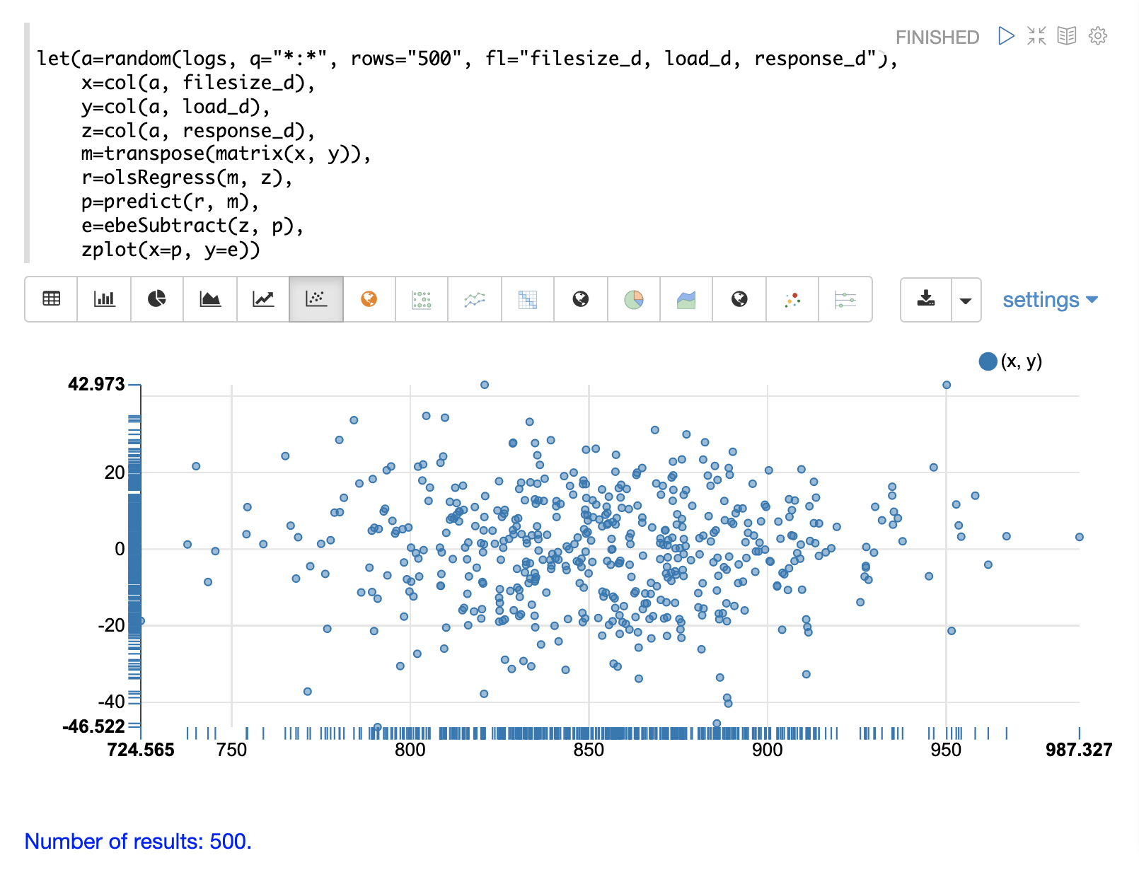
The residual plot for multi-variate linear regression can be interpreted in the exact same way as simple linear regression.