Probability Distributions
This section of the user guide covers the probability distribution framework included in the math expressions library.
Visualization
Probability distributions can be visualized with Zeppelin-Solr using the
zplot function with the dist parameter, which visualizes the
probability density function (PDF) of the distribution.
Example visualizations are shown with each distribution below.
Continuous Distributions
Continuous probability distributions work with continuous numbers (floating points). Below are the supported continuous probability distributions.
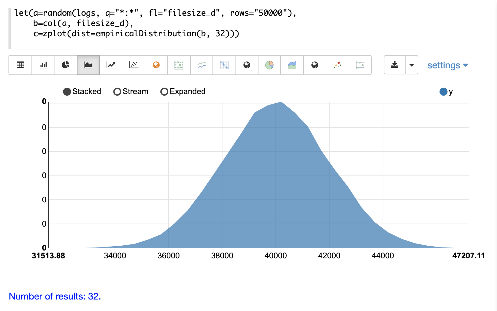
empiricalDistribution
The empiricalDistribution function creates a continuous probability
distribution from actual data.
Empirical distributions can be used to conveniently visualize the probability density function of a random sample from a SolrCloud collection.
The example below shows the zplot function visualizing the probability
density of a random sample with a 32 bin histogram.
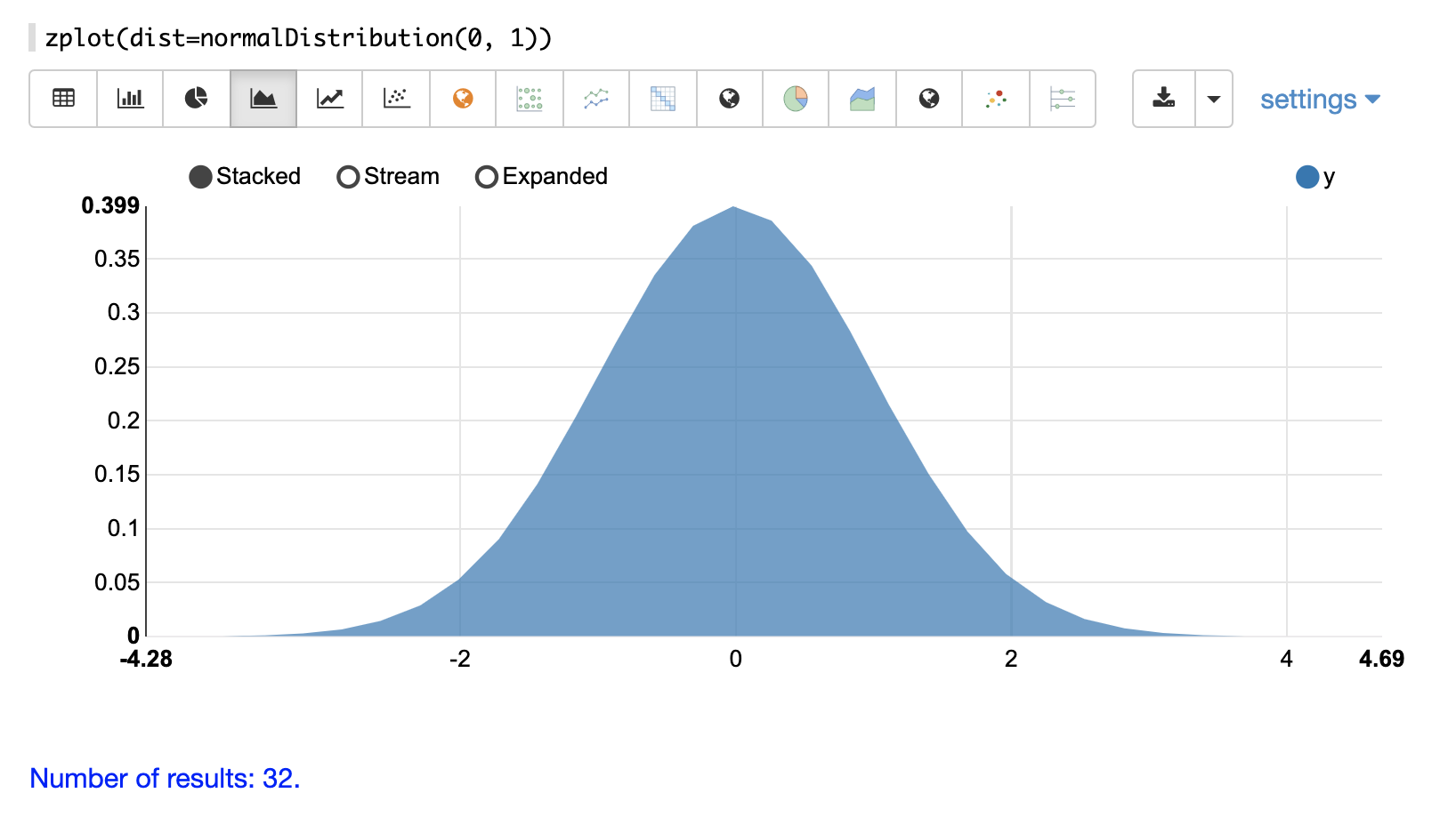
normalDistribution
The visualization below shows a normal distribution with a mean of 0 and standard deviation of 1.
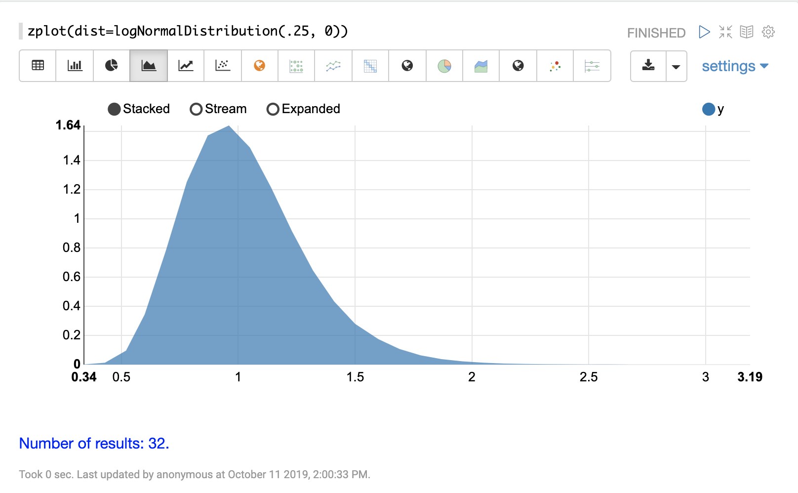
logNormalDistribution
The visualization below shows a log normal distribution with a shape of .25 and scale
of 0.
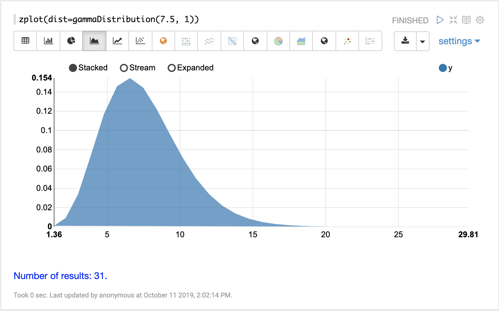
gammaDistribution
The visualization below shows a gamma distribution with a shape of 7.5 and scale
of 1.
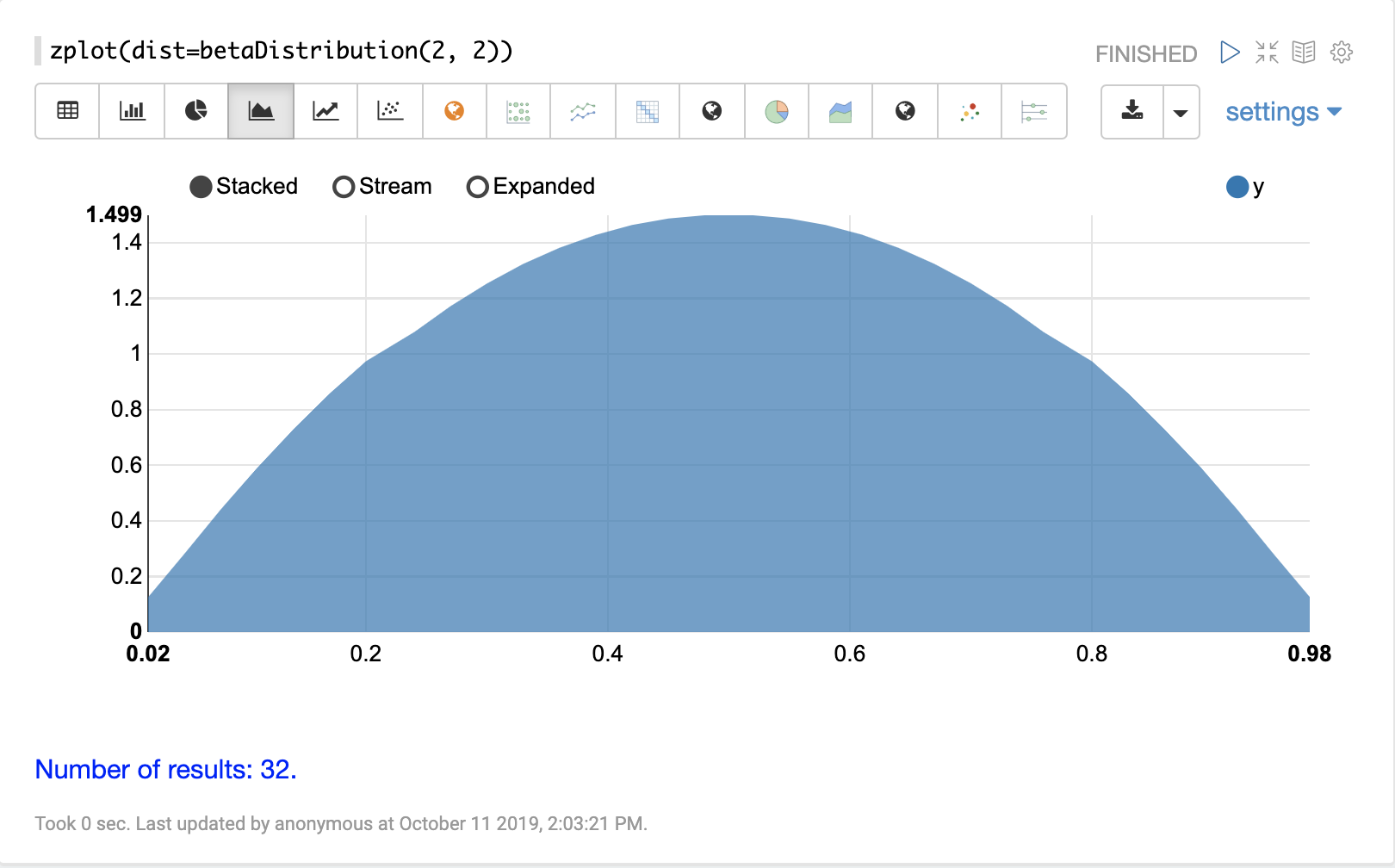
betaDistribution
The visualization below shows a beta distribution with a shape1 of 2 and shape2
of 2.
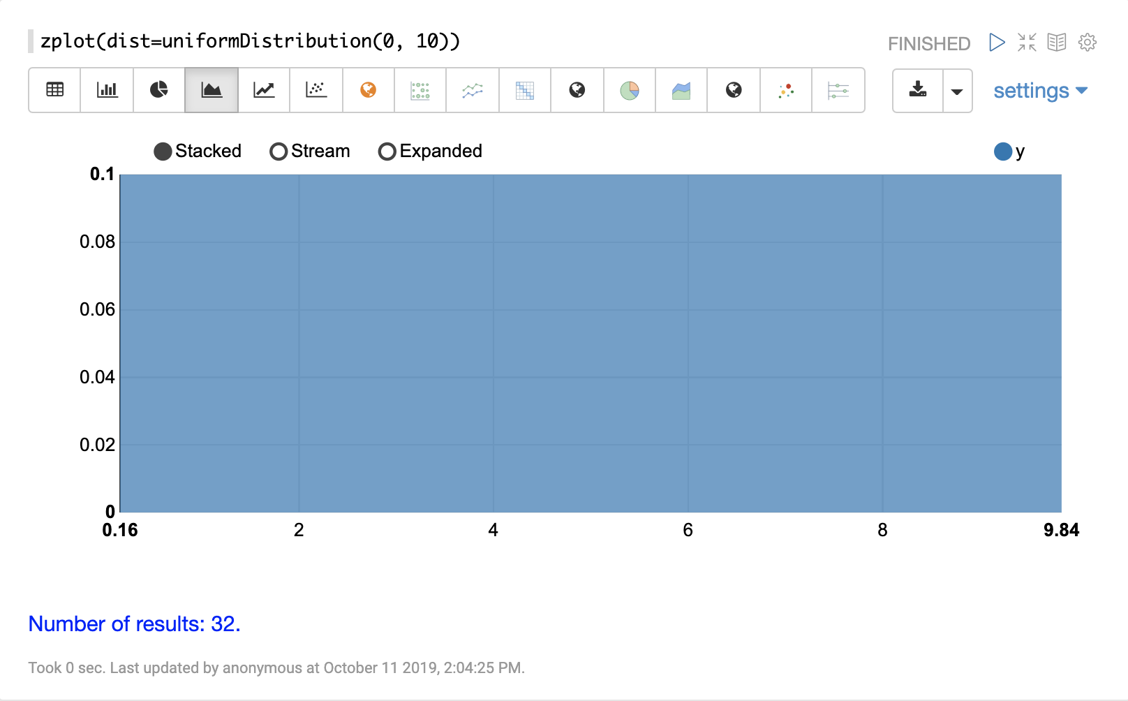
uniformDistribution
The visualization below shows a uniform distribution between 0 and 10.
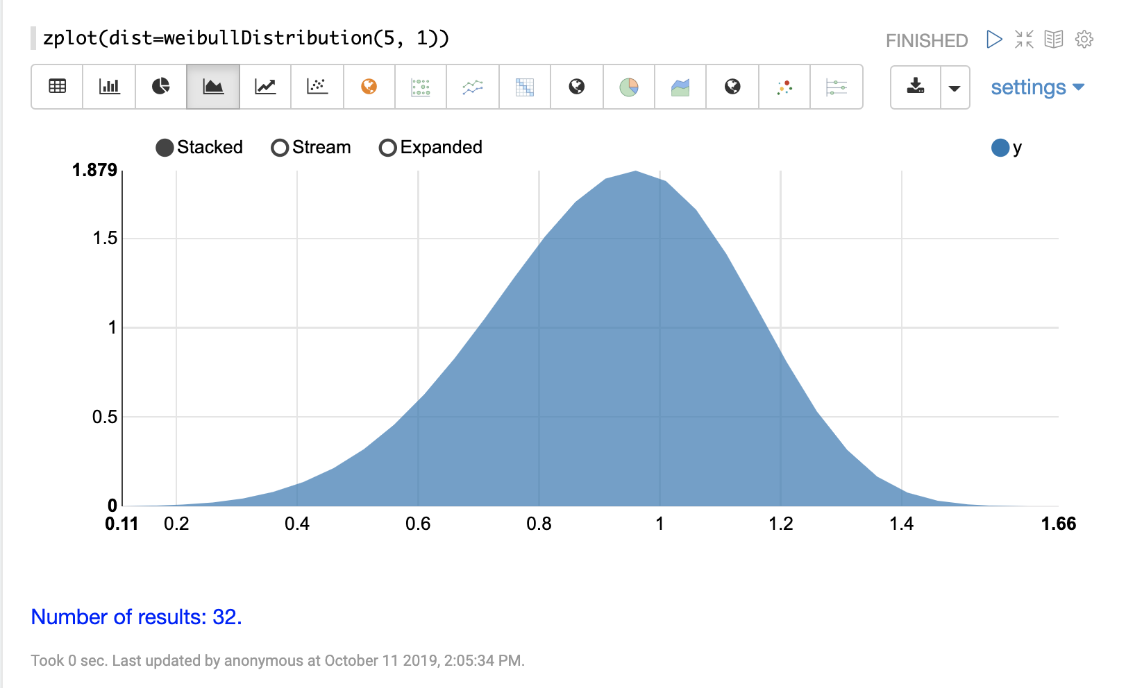
weibullDistribution
The visualization below shows a Weibull distribution with a shape of 5 and scale
of 1.
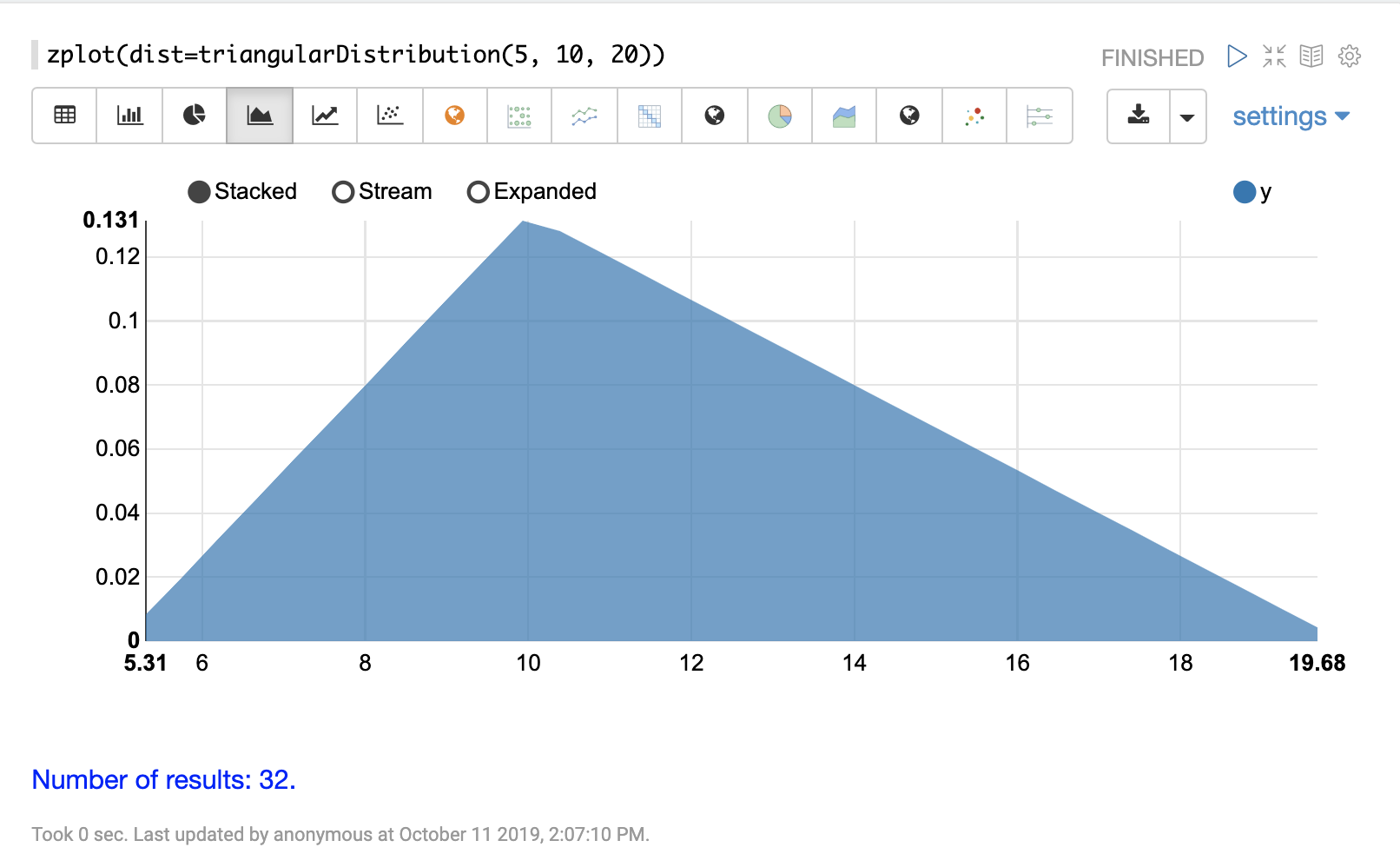
triangularDistribution
The visualization below shows a triangular distribution with a low of 5 a mode of 10 and a high value of 20.
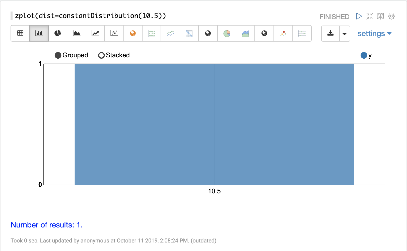
constantDistribution
The visualization below shows a constant distribution of 10.5.
Discrete Distributions
Discrete probability distributions work with discrete numbers (integers). Below are the supported discrete probability distributions.
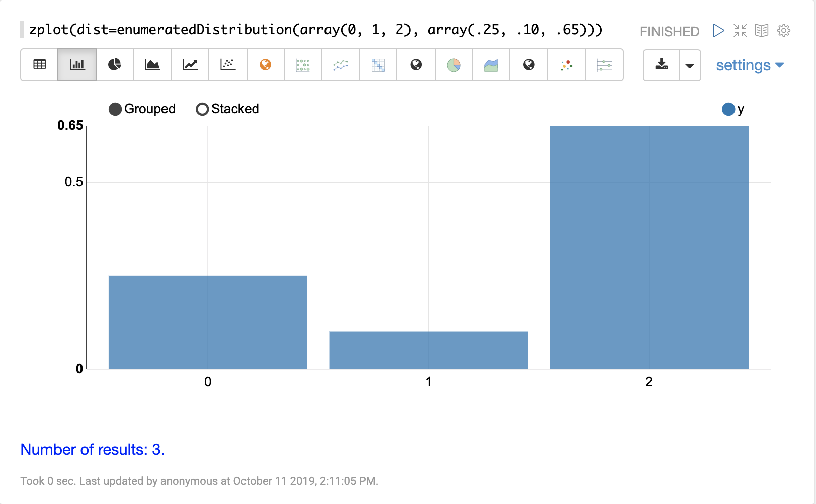
enumeratedDistribution
The enumeratedDistribution function creates a discrete
distribution function
from an enumerated list of values and probabilities or
from a data set of discrete values
The visualization below shows an enumerated distribution created from a list of discrete values and probabilities.
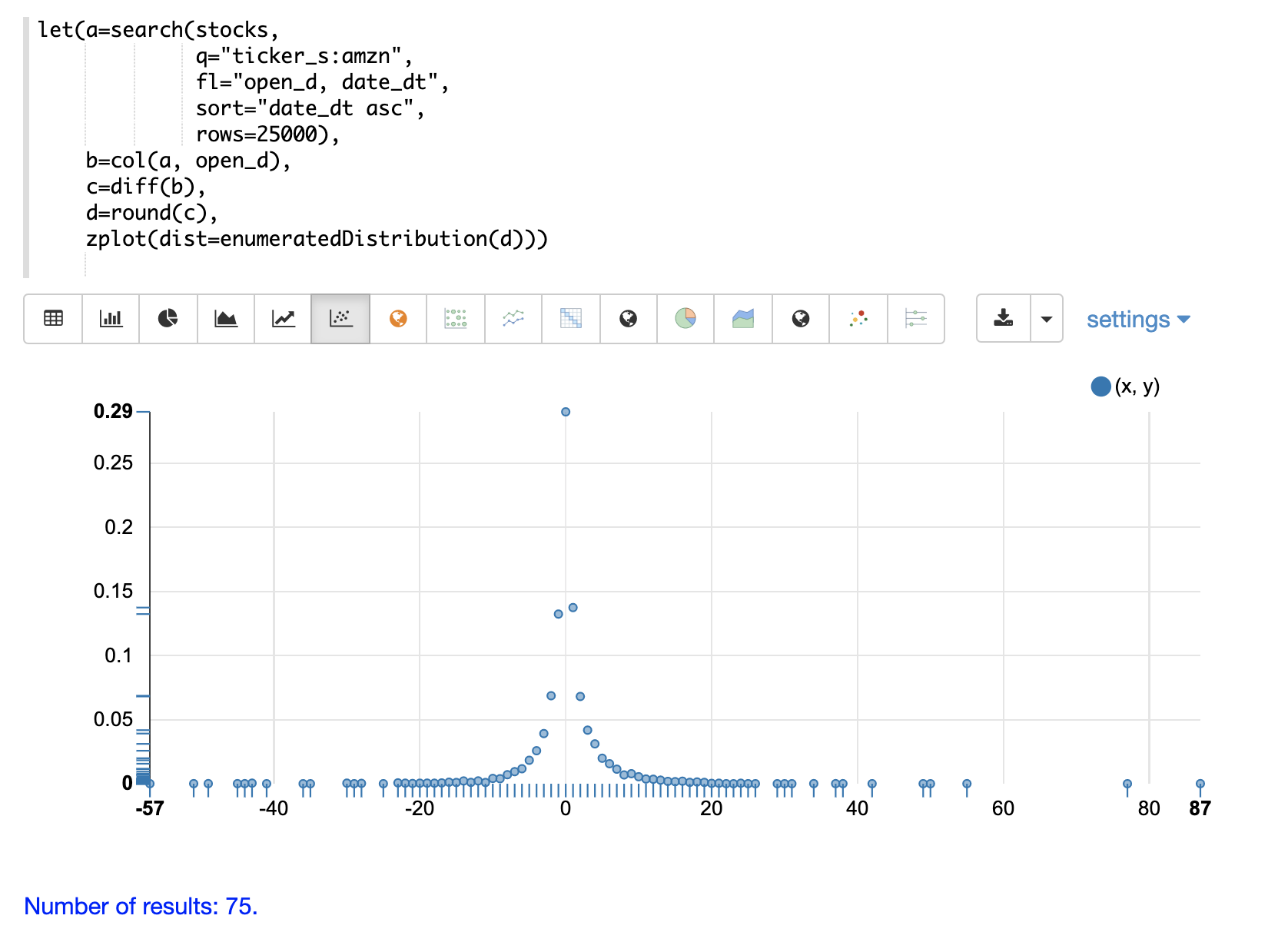
The visualization below shows an enumerated distribution generated from a search result that has been transformed into a vector of discrete values.
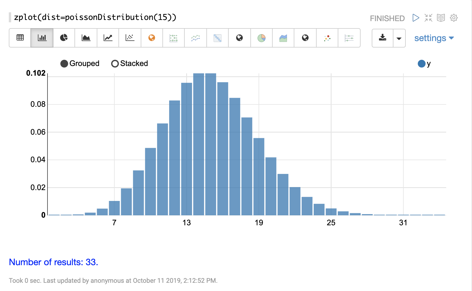
poissonDistribution
The visualization below shows a Poisson distribution with a mean of 15.
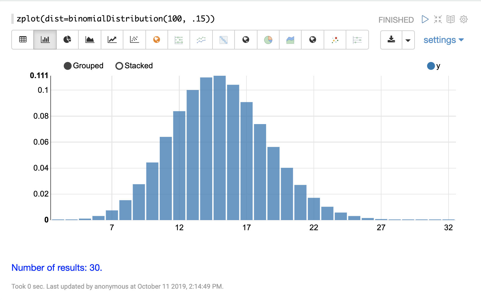
binomialDistribution
The visualization below shows a binomial distribution with a 100 trials and .15 probability of success.
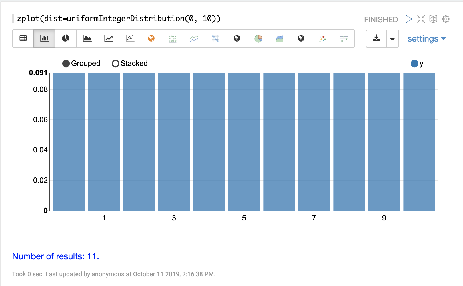
uniformIntegerDistribution
The visualization below shows a uniform integer distribution between 0 and 10.
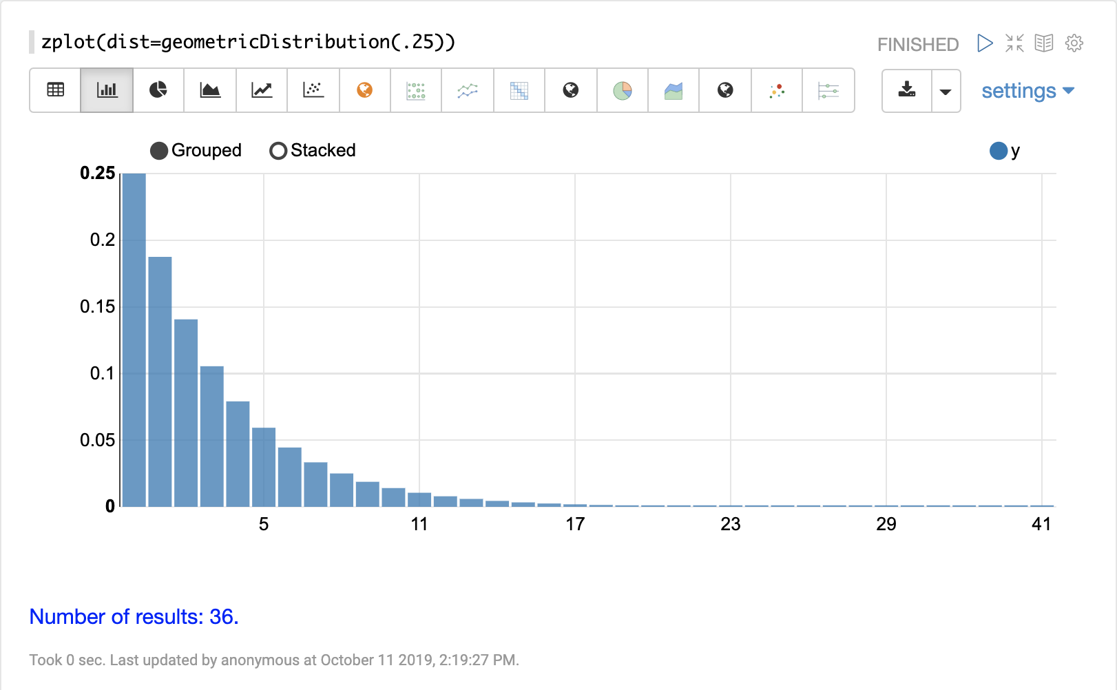
geometricDistribution
The visualization below shows a geometric distribution probability of success of .25.
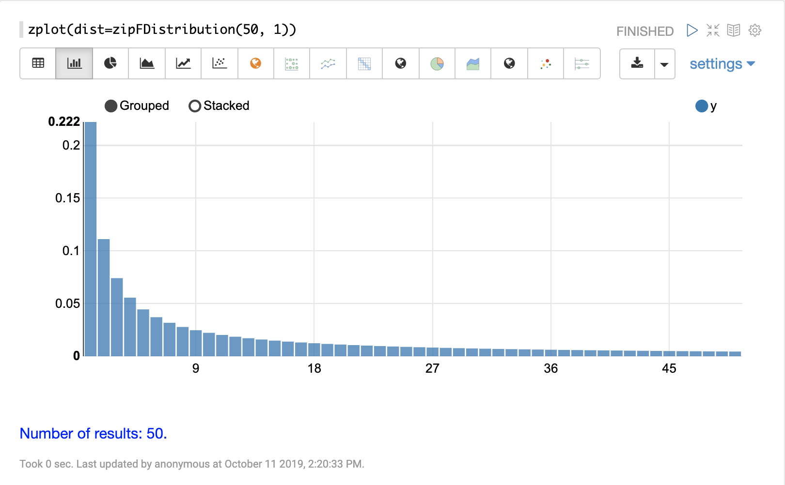
zipFDistribution
The visualization below shows a ZipF distribution with a size of 50 and exponent of 1.
Cumulative Probability
The cumulativeProbability function can be used with all
probability distributions to calculate the
cumulative probability of encountering a specific
random variable within a specific distribution.
Below is example of calculating the cumulative probability of a random variable within a normal distribution.
let(a=normalDistribution(10, 5),
    b=cumulativeProbability(a, 12))
In this example a normal distribution function is created with a mean of 10 and a standard deviation of 5. Then the cumulative probability of the value 12 is calculated for this specific distribution.
When this expression is sent to the /stream handler it responds with:
{
  "result-set": {
    "docs": [
      {
        "b": 0.6554217416103242
      },
      {
        "EOF": true,
        "RESPONSE_TIME": 0
      }
    ]
  }
}
Probability
All probability distributions can calculate the probability between a range of values.
In the following example an empirical distribution is created from a sample of file sizes drawn from the logs collection. Then the probability of a file size between the range of 40000 and 41000 is calculated to be 19%.
let(a=random(logs, q="*:*", fl="filesize_d", rows="50000"),
    b=col(a, filesize_d),
    c=empiricalDistribution(b, 100),
    d=probability(c, 40000, 41000))
When this expression is sent to the /stream handler it responds with:
{
  "result-set": {
    "docs": [
      {
        "d": 0.19006540560734791
      },
      {
        "EOF": true,
        "RESPONSE_TIME": 550
      }
    ]
  }
}
Discrete Probability
The probability function can be used with any discrete
distribution function to compute the probability of a
discrete value.
Below is an example which calculates the probability of a discrete value within a Poisson distribution.
In the example a Poisson distribution function is created
with a mean of 100. Then the
probability of encountering a sample of the discrete value 101 is calculated for this
specific distribution.
let(a=poissonDistribution(100),
    b=probability(a, 101))
When this expression is sent to the /stream handler it responds with:
{
  "result-set": {
    "docs": [
      {
        "b": 0.039466333474403106
      },
      {
        "EOF": true,
        "RESPONSE_TIME": 0
      }
    ]
  }
}
Sampling
All probability distributions support sampling. The sample
function returns one or more random samples from a probability distribution.
Below is an example drawing a single sample from a normal distribution.
let(a=normalDistribution(10, 5),
    b=sample(a))
When this expression is sent to the /stream handler it responds with:
{
  "result-set": {
    "docs": [
      {
        "b": 11.24578055004963
      },
      {
        "EOF": true,
        "RESPONSE_TIME": 0
      }
    ]
  }
}
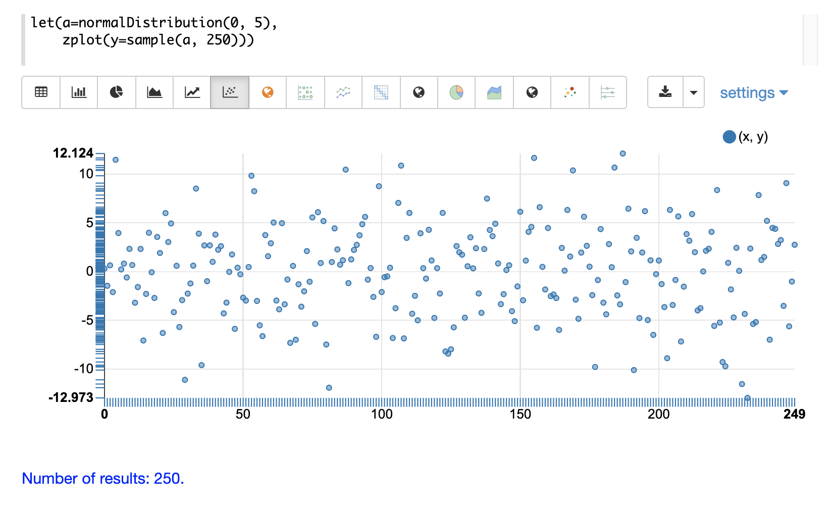
The sample function can also return a vector of samples. Vectors of samples can be visualized as scatter plots to gain an intuitive understanding of the underlying distribution.
The first example shows the scatter plot of a normal distribution with a mean of 0 and a standard deviation of 5.
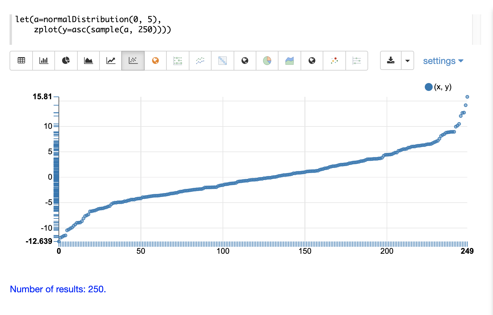
The next example shows a scatter plot of the same distribution with an ascending sort applied to the sample vector.
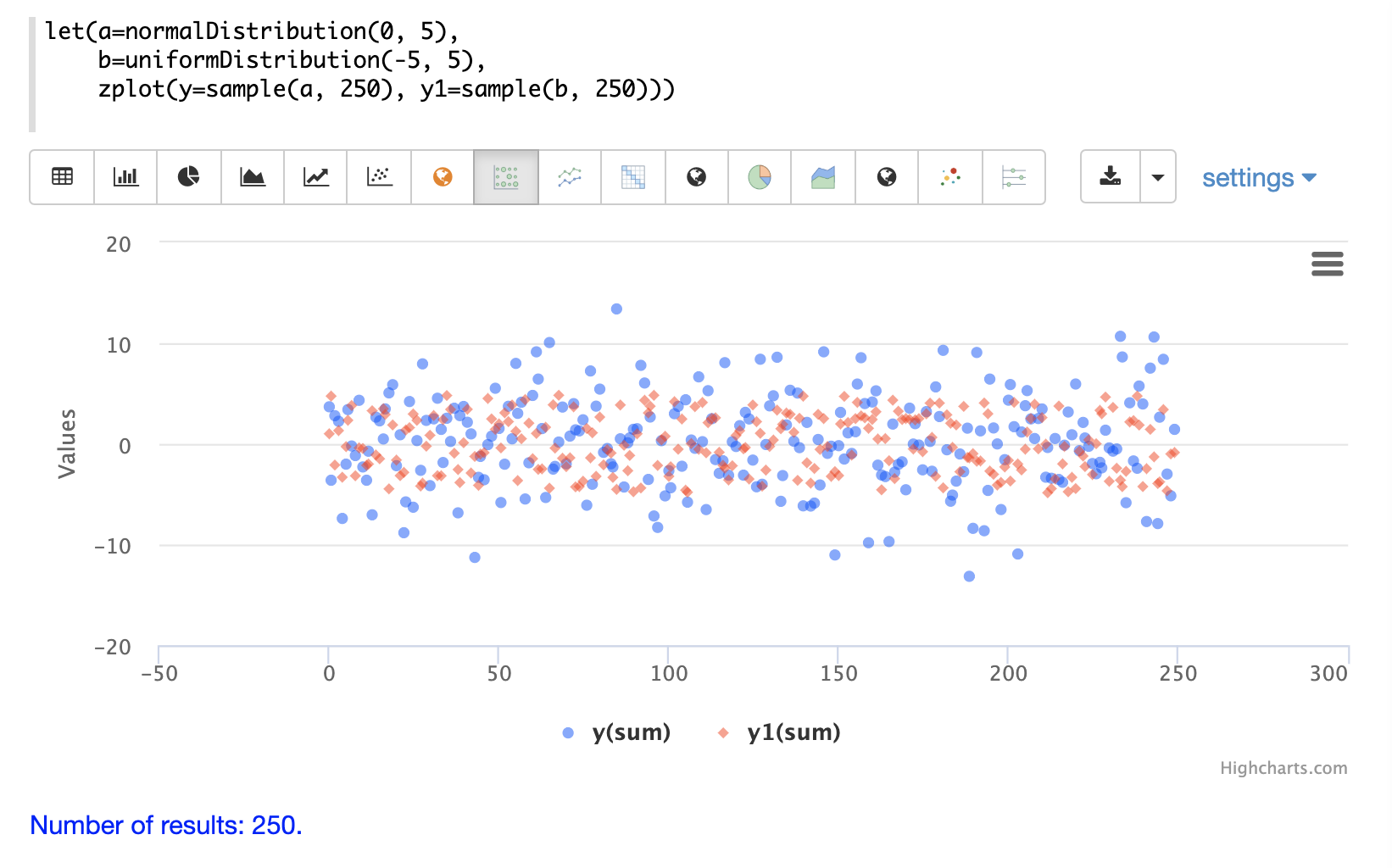
The next example shows two different distributions overlaid in the same scatter plot.
Multivariate Normal Distribution
The multivariate normal distribution is a generalization of the univariate normal distribution to higher dimensions.
The multivariate normal distribution models two or more random variables that are normally distributed. The relationship between the variables is defined by a covariance matrix.
Sampling
The sample function can be used to draw samples
from a multivariate normal distribution in much the same
way as a univariate normal distribution.
The difference is that each sample will be an array containing a sample
drawn from each of the underlying normal distributions.
If multiple samples are drawn, the sample function returns a matrix with a
sample in each row. Over the long term the columns of the sample
matrix will conform to the covariance matrix used to parametrize the
multivariate normal distribution.
The example below demonstrates how to initialize and draw samples from a multivariate normal distribution.
In this example 5000 random samples are selected from a collection of log records. Each sample contains
the fields filesize_d and response_d. The values of both fields conform to a normal distribution.
Both fields are then vectorized. The filesize_d vector is stored in
variable b and the response_d variable is stored in variable c.
An array is created that contains the means of the two vectorized fields.
Then both vectors are added to a matrix which is transposed. This creates
an observation matrix where each row contains one observation of
filesize_d and response_d. A covariance matrix is then created from the columns of
the observation matrix with the cov function. The covariance matrix describes the covariance between
filesize_d and response_d.
The multivariateNormalDistribution function is then called with the
array of means for the two fields and the covariance matrix. The model for the
multivariate normal distribution is assigned to variable g.
Finally five samples are drawn from the multivariate normal distribution.
let(a=random(logs, q="*:*", rows="5000", fl="filesize_d, response_d"),
    b=col(a, filesize_d),
    c=col(a, response_d),
    d=array(mean(b), mean(c)),
    e=transpose(matrix(b, c)),
    f=cov(e),
    g=multiVariateNormalDistribution(d, f),
    h=sample(g, 5))
The samples are returned as a matrix, with each row representing one sample. There are two
columns in the matrix. The first column contains samples for filesize_d and the second
column contains samples for response_d. Over the long term the covariance between
the columns will conform to the covariance matrix used to instantiate the
multivariate normal distribution.
{
  "result-set": {
    "docs": [
      {
        "h": [
          [
            41974.85669321393,
            779.4097049705296
          ],
          [
            42869.19876441414,
            834.2599296790783
          ],
          [
            38556.30444839889,
            720.3683470060988
          ],
          [
            37689.31290928216,
            686.5549428100018
          ],
          [
            40564.74398214547,
            769.9328090774
          ]
        ]
      },
      {
        "EOF": true,
        "RESPONSE_TIME": 162
      }
    ]
  }
}