Curve Fitting
These functions support constructing a curve through bivariate non-linear data.
Polynomial Curve Fitting
The polyfit function is a general purpose curve fitter used to model
the non-linear relationship between two random variables.
The polyfit function is passed x- and y-axes and fits a smooth curve to the data.
If only a single array is provided it is treated as the y-axis and a sequence is generated
for the x-axis. A third parameter can be added that specifies the degree of the polynomial. If the degree is
not provided a 3 degree polynomial is used by default. The higher
the degree the more curves that can be modeled.
The polyfit function can be visualized in a similar manner to linear regression with
Zeppelin-Solr.
The example below uses the polyfit function to fit a non-linear curve to a scatter
plot of a random sample. The blue points are the scatter plot of the original observations and the red points
are the predicted curve.
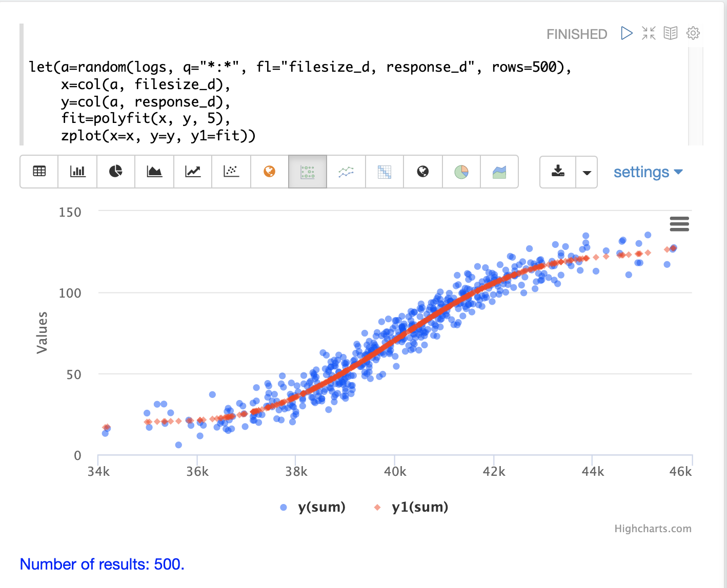
In the example above a random sample containing two fields, filesize_d
and response_d, is drawn from the logs collection.
The two fields are vectorized and set to the variables x and y.
Then the polyfit function is used to fit a non-linear model to the data using a 5 degree
polynomial. The polyfit function returns a model that is then directly plotted
by zplot along with the original observations.
The fitted model can also be used
by the predict function in the same manner as linear regression. The example below
uses the fitted model to predict a response time for a file size of 42000.
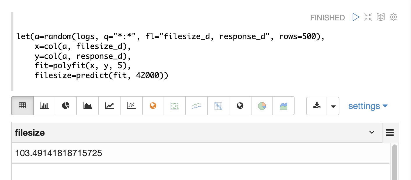
If an array of predictor values is provided an array of predictions will be returned.
The polyfit model performs both interpolation and extrapolation,
which means that it can predict results both within the bounds of the data set
and beyond the bounds.
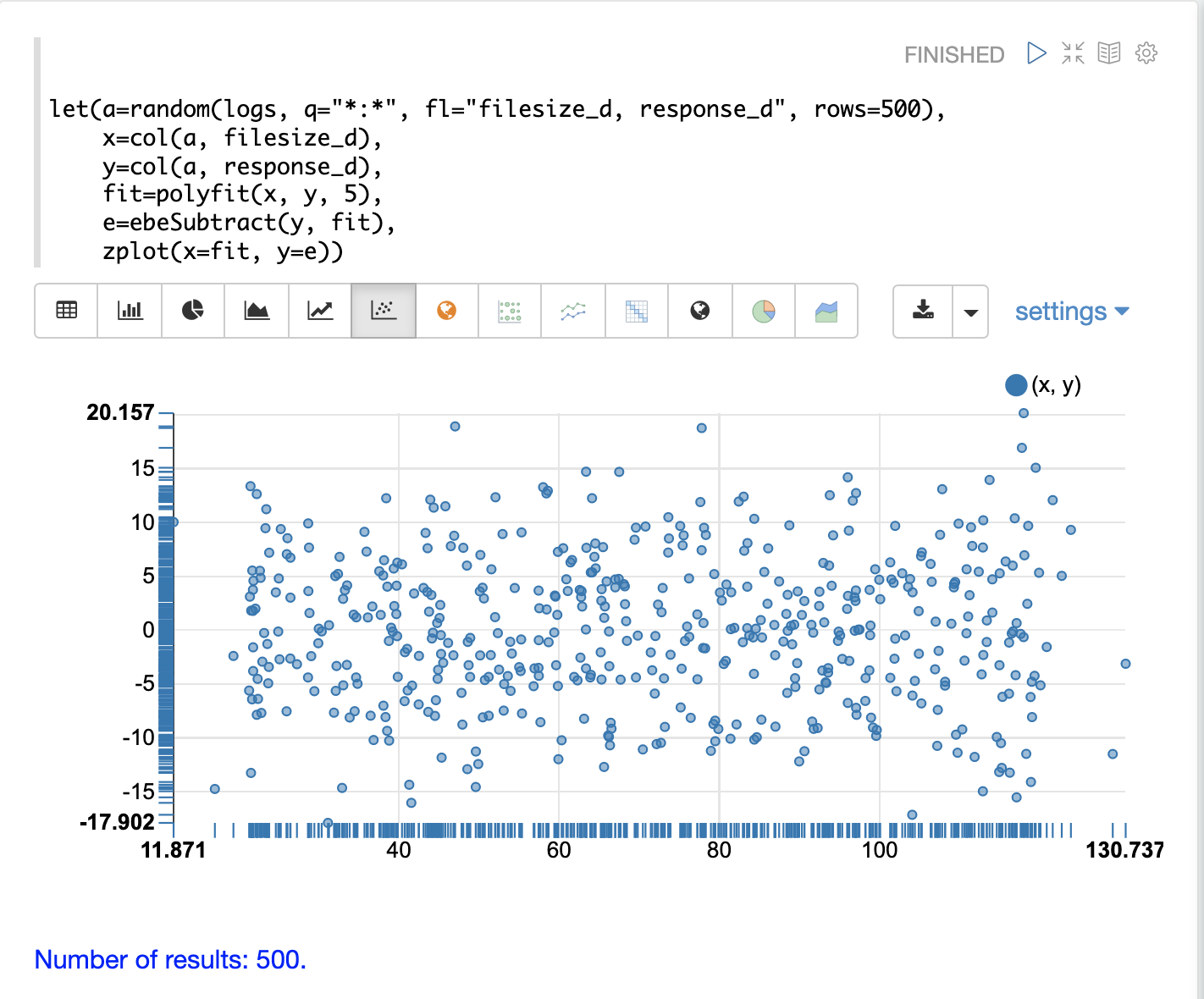
Residuals
The residuals can be calculated and visualized in the same manner as linear
regression as well. In the example below the ebeSubtract function is used
to subtract the fitted model from the observed values, to
calculate a vector of residuals. The residuals are then plotted in a residual plot
with the predictions along the x-axis and the model error on the y-axis.
Gaussian Curve Fitting
The gaussfit function fits a smooth curve through a Gaussian peak. The gaussfit
function takes an x- and y-axis and fits a smooth gaussian curve to the data. If
only one vector of numbers is passed, gaussfit will treat it as the y-axis
and will generate a sequence for the x-axis.
One of the interesting use cases for gaussfit is to visualize how well a regression
model’s residuals fit a normal distribution.
One of the characteristics of a well-fit regression model is that its residuals will ideally fit a normal distribution. We can test this by building a histogram of the residuals and then fitting a gaussian curve to the curve of the histogram.
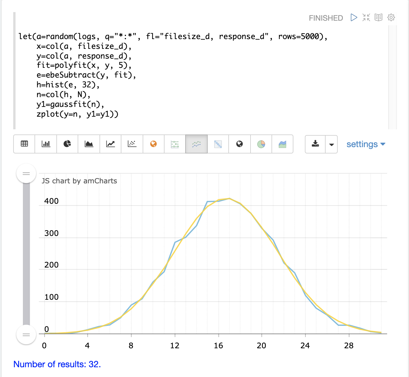
In the example below the residuals from a polyfit regression are modeled with the
hist function to return a histogram with 32 bins. The hist function returns
a list of tuples with statistics about each bin. In the example the col function is
used to return a vector with the N column for each bin, which is the count of
observations in the
bin. If the residuals are normally distributed we would expect the bin counts
to roughly follow a gaussian curve.
The bin count vector is then passed to gaussfit as the y-axis. gaussfit generates
a sequence for the x-axis and then fits the gaussian curve to data.
zplot is then used to plot the original bin counts and the fitted curve. In the
example below, the blue line is the bin counts, and the smooth yellow line is the
fitted curve. We can see that the binned residuals fit fairly well to a normal
distribution.
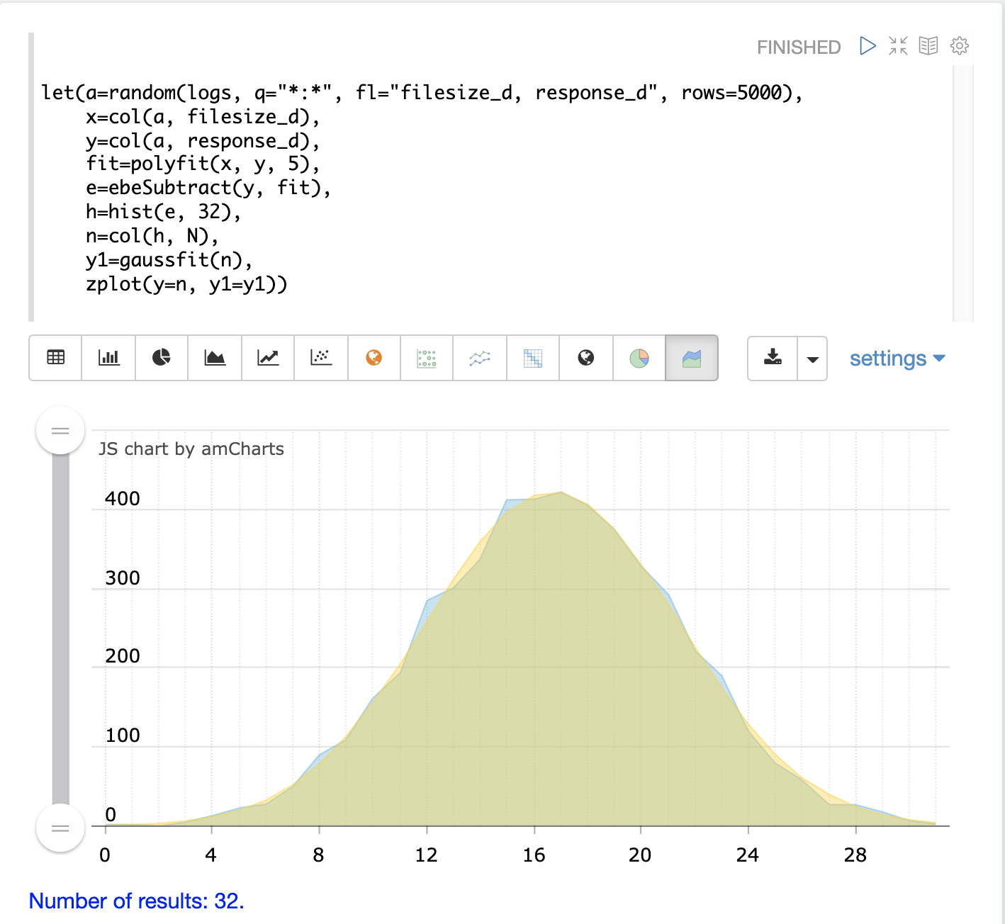
The second plot shows the two curves overlaid with an area chart:
Harmonic Curve Fitting
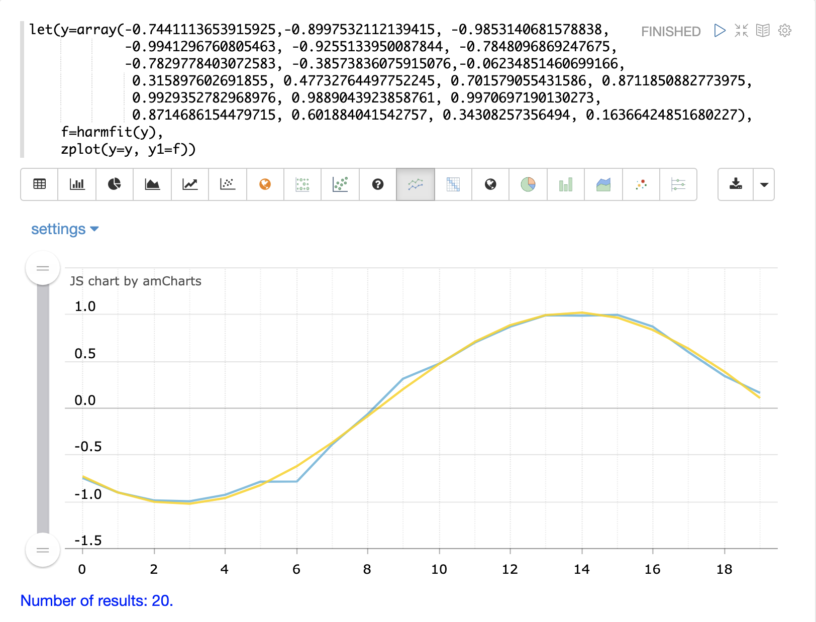
The harmonicFit function (or harmfit, for short) fits a smooth line through control points of a sine wave.
The harmfit function is passed x- and y-axes and fits a smooth curve to the data.
If a single array is provided it is treated as the y-axis and a sequence is generated
for the x-axis.
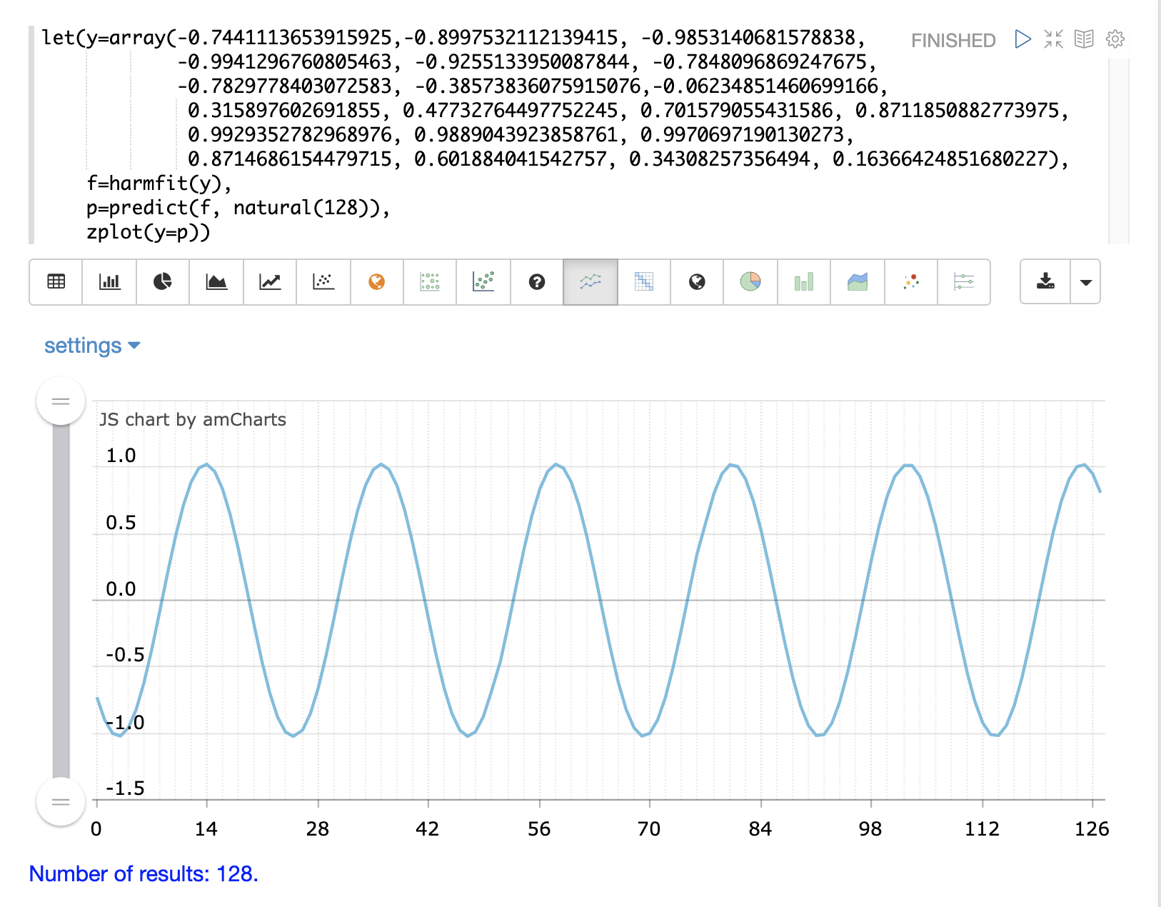
The example below shows harmfit fitting a single oscillation of a sine wave. The harmfit function
returns the smoothed values at each control point. The return value is also a model which can be used by
the predict, derivative and integrate functions.
The harmfit function works best when run on a single oscillation rather than a long sequence of
oscillations. This is particularly true if the sine wave has noise. After the curve has been fit it can be
extrapolated to any point in time in the past or future.
|
In the example below the original control points are shown in blue and the fitted curve is shown in yellow.
The output of harmfit is a model that can be used by the predict function to interpolate and extrapolate
the sine wave. In the example below the natural function creates an x-axis from 0 to 127
used to predict results for the model. This extrapolates the sine wave out to 128 points, when
the original model curve had only 19 control points.